Week 5 - Curve fitting

Curve Fitting is the process of fitting actual data with a function that can be used to predict behaviour outside the domain of the actual data. In order to do this many types of functions can be used such as linear, quadratic, exponential, cubic etc. The following program shows how Python can be used to fit actual temperature and Cp data with the appropriate function.

popt - Returns optimal values for the parameters so that the sum of the squared residuals of f(xdata, *popt) - ydata is minimized.

pcov - It is the estimated covariance of popt. The diagonals provide the variance of the parameter estimate.

np.array(Temperature) - This is used to input the temperature array to a function.

*popt - popt stores the optimal value of coefficients a,b,c after curve fitting. Using the * inputs all these values into the curve_fit function

import matplotlib.pyplot as plt
from scipy.optimize import curve_fit
import numpy as np

# Linear Function
def lin_func(t,a,b):
	return a*t + b

# Quadratic Function
def quad_func(t,a,b,c):
	return a*pow(t,2) + b*t + c

# Cubic function
def cub_func(t,a,b,c,d):
	return a*pow(t,3) + b*pow(t,2) + c*t + d

# Reading the data file
def read_file():
	Temperature = []
	Cp = []
	for line in open('data','r'):
		values = line.split(',')
		Temperature.append(float(values[0]))
		Cp.append(float(values[1]))
	return [Temperature, Cp]

# Main Program
Temperature, Cp = read_file()
lin_popt, lin_pcov = curve_fit(lin_func, Temperature, Cp)
lin_fit_Cp = lin_func(np.array(Temperature), *lin_popt)

quad_popt, quad_pcov = curve_fit(quad_func, Temperature, Cp)
quad_fit_Cp = quad_func(np.array(Temperature), *quad_popt)

cub_popt, cub_pcov = curve_fit(cub_func, Temperature, Cp)
cub_fit_Cp = cub_func(np.array(Temperature), *cub_popt)

def r2(y,f):
	# residual sum of squares
	ss_res = np.sum((y - f) ** 2)

	# total sum of squares
	ss_tot = np.sum((y - np.mean(y)) ** 2)

	# r-squared
	r2 = 1 - (ss_res / ss_tot)
	return r2

lin_r2 = r2(Cp,lin_fit_Cp)
quad_r2 = r2(Cp,quad_fit_Cp)
cub_r2 = r2(Cp,cub_fit_Cp)

# Plotting both functions
plt.figure()
plt.plot(Temperature, Cp, color = "blue", lw= 2)
plt.plot(Temperature, lin_fit_Cp, color = "red", lw=2)
plt.legend(['Actual data','Linear Curve Fit'])
plt.xlabel('Temperature [K]')
plt.ylabel('Cp')

plt.figure()
plt.plot(Temperature, Cp, color = "blue", lw= 2)
plt.plot(Temperature, quad_fit_Cp, color = "red", lw=2)
plt.legend(['Actual data','Quadratic Curve Fit'])
plt.xlabel('Temperature [K]')
plt.ylabel('Cp')

plt.figure()
plt.plot(Temperature, Cp, color = "blue", lw= 2)
plt.plot(Temperature, cub_fit_Cp, color = "red", lw=2)
plt.legend(['Actual data','Cubic Curve Fit'])
plt.xlabel('Temperature [K]')
plt.ylabel('Cp')
plt.show()

print('Goodness of linear fit is :', lin_r2)
print('Goodness of quadratic fit is :', quad_r2)
print('Goodness of cubicr fit is :', cub_r2)

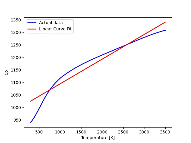
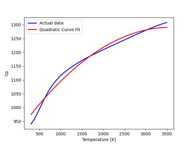
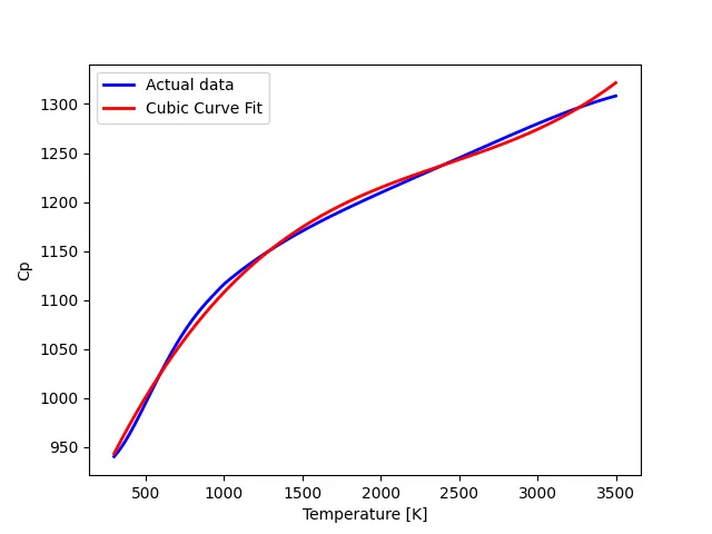
The different fits can be seen below

Linear Fit:

Quadratic Fit:

Cubic Fit:

The empirical goodness of fit was calculated using the R-squared method. A function was created and the R-square value for all three fits was calculated and the results are as shown below

Clearly we can see that the cubic polynomial function showed the best fit. However, for a better fit the temperature range could be split into low-temperature and high-temperature range resulting in a better fit.