Week 4 - Genetic Algorithm

A genetic algorithm is an optimization algorithm that is inspired by Charles Darwin’s theory of natural evolution. This algorithm reflects the process of natural selection where the fittest individuals are selected for reproduction in order to produce offspring of the next generation. In this process, natural selection starts with the selection of fittest individuals from a population. They produce offspring which inherit the characteristics of the parents and will be added to the next generation. If parents have better fitness, their offspring will be better than parents and have a better chance at surviving. This process keeps on iterating and at the end, a generation with the fittest individuals will be found.

Genetic Algorithm consists of 5 phases

Initial Population - The process begins with a set of individuals which is called a Population. Each individual is a solution to the problem you want to solve.

Fitness Function - The fitness function determines how fit an individual is (the ability of an individual to compete with other individuals). It gives a fitness score to each individual. The probability that an individual will be selected for reproduction is based on its fitness score.

Selection - The selection phase involves selecting the fittest individuals and letting them pass their genes to the next generation. Two pairs of individuals (parents) are selected based on their fitness scores. Individuals with high fitness have more chance to be selected for reproduction.

Crossover - It is the most significant phase in a genetic algorithm. For each pair of parents to be mated, a crossover point is chosen at random from within the genes by mutating the old generation parents.

Mutation - In certain new offspring formed, some of their genes can be subjected to a mutation with a low random probability. This implies that some of the bits in the bit string can be flipped.

Syntax

x = ga(fun,vars)

The above syntax finds the local unconstrained minimum x, to the objective function, fun. nvars is the number of variables to the function, fun.

First a random array of x,y were created using meshgrid command. A nested loop was used to assign values from this array into an array named input_vector. The input_vector array was passed as input to the stalagmite function which is coded separately. 4 cases are considered when using the ga command. tic-toc commands were used to measure the time taken for ga to optimize the stalagmite function for each case. The first case involved using basic ga command with initial population of 50 and no bounds of search. The second case involved setting a certain bound to the search space within which one can expect to find the maxima. The third and fourth cases involved further increase in population size to 100 and 300 respectively to accurately locate the maxima. As we know ga gives different results every time it is run, it is important to define our search space in order to locate the most reasonable and correct maxima. surfc command was used to plot the stalagmite function and plot3 command was used to plot the results. The trick here was to code the stalagmite function in such a way that we obtain maximum and not minimum value. As we know ga always finds the minima of a function, the stalagmite function was negated as in -f, so that we could obtain the maxima of the function. The same was done while plotting in order to visualize the result better.

Main Program:

clear all 
close all
clc

x = linspace(0,0.6,150);
y = linspace(0,0.6,150);
num_cases = 50;

[xx yy] = meshgrid(x,y);

for i = 1:length(xx)
    for j = 1:length(yy)
        input_vector(1) = xx(i,j);
        input_vector(2) = yy(i,j);
        f(i,j) = stalagmite(input_vector);
    end 
end
tic
for i = 1:num_cases
    [inputs, fopt(i)] = ga(@stalagmite, 2);
    xopt(i) = inputs(1);
    yopt(i) = inputs(2);
end
case_time_1 = toc
figure(1)
subplot(2,1,1)
hold on
surfc(xx,yy,-f)
shading interp
plot3(xopt,yopt,-fopt,'marker','o','markersize',5,'markerfacecolor','r');
subplot(2,1,2)
plot(-fopt)
xlabel('Iterations')
ylabel('Function Minimum')


%Case 2 With bounds
tic
for i = 1:num_cases
    [inputs, fopt(i)] = ga(@stalagmite, 2,[],[],[],[],[0;0],[0.6;0.6]);
    xopt(i)=inputs(1);
    yopt(i)=inputs(2);
end
case_time_2 = toc
figure(2)
subplot(2,1,1)
hold on
surfc(xx,yy,-f)
shading interp
plot3(xopt,yopt,-fopt,'marker','o','markersize',5,'markerfacecolor','r');
subplot(2,1,2)
plot(-fopt)
xlabel('Iterations')
ylabel('Function Minimum')

%Case 3 With bounds and increasing number of cases to 100

options = optimoptions('ga');
options = optimoptions(options,'populationsize',100);

tic
for i=1:num_cases
    [inputs,fopt(i)] = ga(@stalagmite,2,[],[],[],[],[0;0],[0.6;0.6],[],[],options);
    xopt(i)=inputs(1);
    yopt(i)=inputs(2);
end
case_time_3 = toc
figure(3)
subplot(2,1,1)
hold on
surfc(xx,yy,-f)
shading interp
plot3(xopt,yopt,-fopt,'marker','o','markersize',5,'markerfacecolor','r');
subplot(2,1,2)
plot(-fopt)
xlabel('Iterations')
ylabel('Function Minimum')

%Case 4: Increasing population to 300
options = optimoptions('ga');
options = optimoptions(options,'populationsize',300);
tic
for i=1:num_cases
    [inputs,fopt(i)] = ga(@stalagmite,2,[],[],[],[],[0;0],[0.1;0.1],[],[],options);
    xopt(i)=inputs(1);
    yopt(i)=inputs(2);
end
case_time_4 = toc
figure(4)
subplot(2,1,1)
hold on
surfc(xx,yy,-f)
shading interp
plot3(xopt,yopt,-fopt,'marker','o','markersize',5,'markerfacecolor','r');
subplot(2,1,2)
plot(-fopt)
xlabel('Iterations')
ylabel('Function Minimum')

Stalagmite Function Code:

function [f] = stalagmite(input_vector)
    
    f1x = (sin((input_vector(1)*pi*5.1) + 0.5)).^6;
    f1y = (sin((input_vector(2)*pi*5.1) + 0.5)).^6;
    f2x = exp(-(4*log(2)*((input_vector(1) - 0.0667).^2))/(0.64));
    f2y = exp(-(4*log(2)*((input_vector(2) - 0.0667).^2))/(0.64));
    f1 = f1x.*f1y.*f2x.*f2y;
    f = -f1;
end

Results:

Case 1: Unbounded

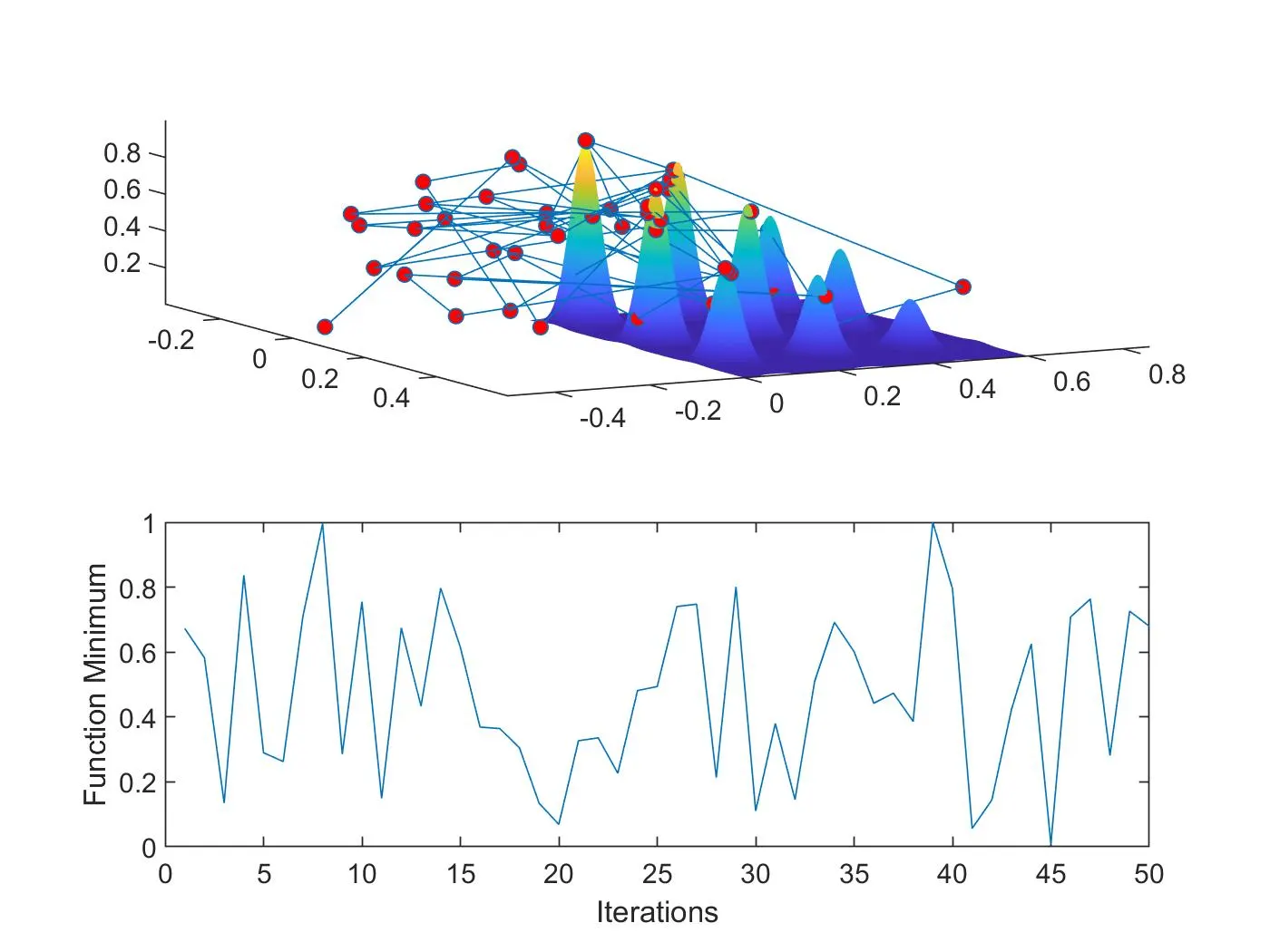
Case 2: Bounded

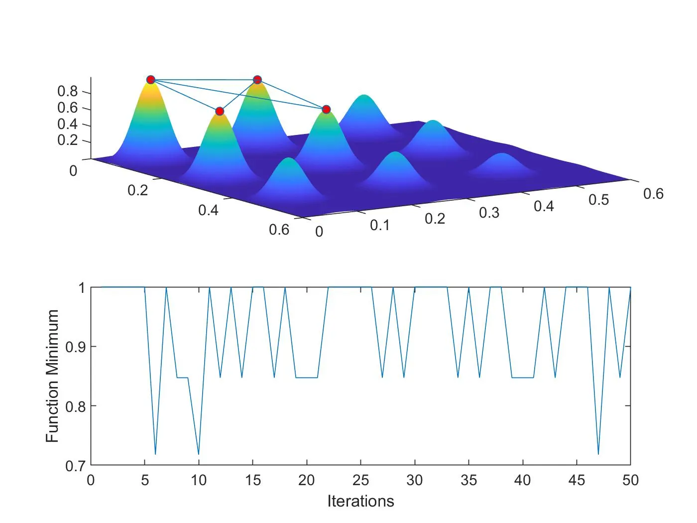
Case 3: Bounded with population of 100

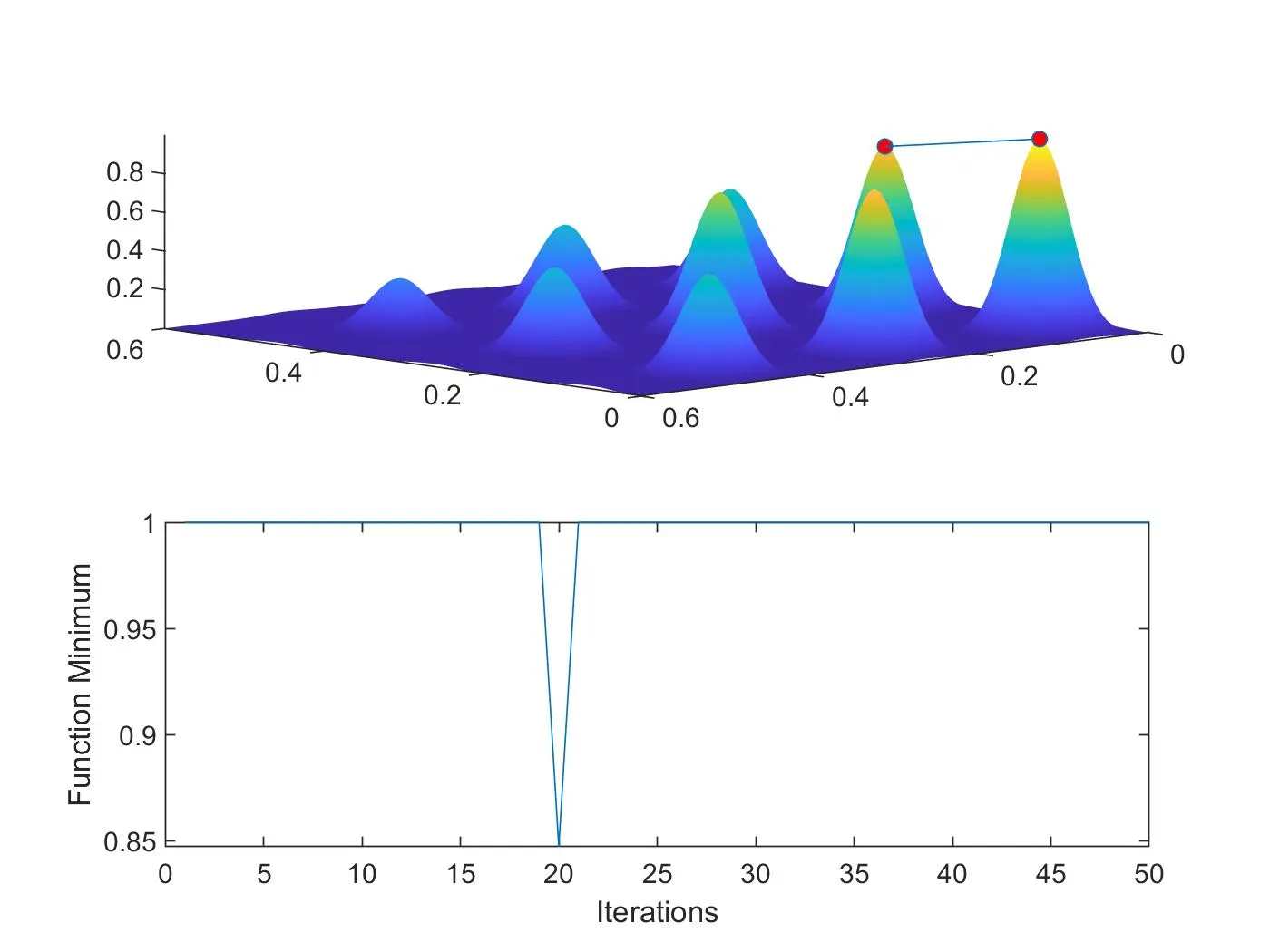
Case 4: Bounded with population of 300

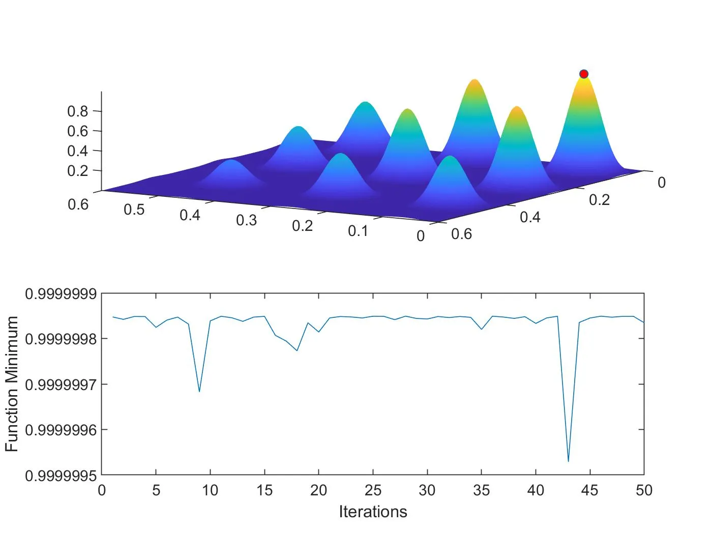
Values of x & y at which stalagmite function reaches maximum:

x = 0.0668, y = 0.0668