Week 3 - Solving second order ODEs

In engineering practices, ordinary differential equations are used to describe the transient behaviour of a system. In this case, the behaviour of a simple pendulum can be modelled with the following differential equation

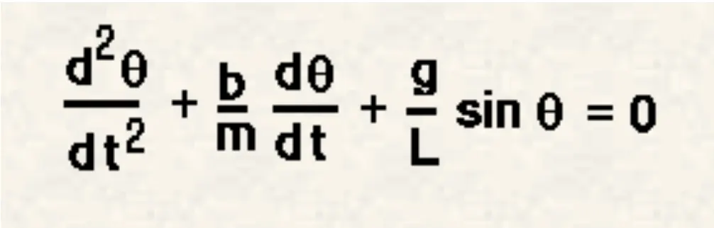
The above equation can be simplified into a system of first order differential equations which are then solved using 'odeint' from the 'scipy.integrate' library. The python code is shown below

import numpy as np
import math 
import matplotlib.pyplot as plt
from scipy.integrate import odeint
import matplotlib.animation as animation

# Defining the function which contains the set of differential equations to solve
def model(theta,t,b,g,l,m):
	theta1 = theta[0]
	theta2 = theta[1]
	dtheta1_dt = theta2
	dtheta2_dt = -(b/m)*theta2 - (g/l)*math.sin(theta1)
	dtheta_dt = [dtheta1_dt, dtheta2_dt]
	return dtheta_dt

# Pendulum Inputs
# Damping Co-efficient
b = 0.05
# Length of string
l = 1
# Gravity
g = 9.81
# Mass of bob
m = 1
# Initial conditions
theta_0 = [0,3]
# Defining time array
t = np.linspace(0,20,150)

# Solving the ODE
theta = odeint(model,theta_0,t,args = (b,g,l,m))

# Plotting transient behaviour
plt.figure()
plt.plot(t,theta[:,0],'b-',label = r'$\frac{d\theta1}{dt}=\theta2$, Displacement')
plt.plot(t,theta[:,1],'r--',label = r'$\frac{d\theta2}{dt}=\frac{b}{m}\theta2-\frac{g}{l}sin\theta_1$, Velocity')
plt.xlabel('Time')
plt.ylabel('Plot')
plt.xlim(0,22)
plt.ylim(-4.5,4.5)
plt.legend(loc='upper right')
plt.show()

# Animating the pendulum motion
fig = plt.figure(figsize = (5,5), facecolor = 'w')
ax = fig.add_subplot(1,1,1)
plt.rcParams['font.size'] = 15

tmp = []
for i in range(len(theta)):

	# Plotting horizontal line
	hl, = ax.plot([-0.5,0.5],[0,0],'k',linewidth = 3)

	# Plotting the string/chord
	ln, = ax.plot([0, np.sin(theta[i,0])], [0, -np.cos(theta[i,0])],color='k',lw=2)

	# Plotting the bob
	bob, = ax.plot(np.sin(theta[i,0]),-np.cos(theta[i,0]),'o',markersize = 20,color = 'r')

	# Plotting the time for simulation
	tm = ax.text(-0.5,0.25, 'Time = %.1fs' % t[i])
	tmp.append([hl,ln,bob,tm])

ax.set_aspect('equal','datalim')

# Saving the animation
ani = animation.ArtistAnimation(fig,tmp,interval = 50)
fn = 'Pendulum Animation'
ani.save(fn+'.mp4',writer='ffmpeg',fps=1000/50)

The 2 first order ODE's are defined in a function which is then called to the 'odeint' solver. The results of angular position and velocity are plotted using 'matplotlib.pyplot' as shown below

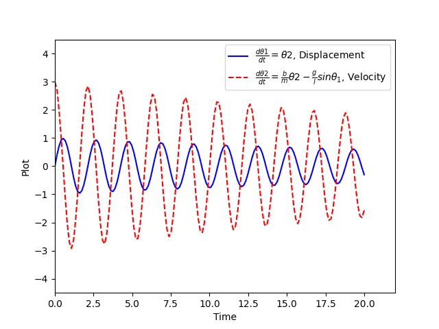
From the plot we can see that the angular position or theta was initially zero and keeps reducing due to the damping factor 'b'. Similarly the angular velocity starts at 3 rad/s which is our initial condition and then slowly gets damped which can be seen from the reduced amplitudes.

The animation of the simple pendulum motion was created using 'matplotlib.animation' library. Artist.animation is used to generate animation from the 'for' loop plotting the string and bob for each position of the pendulum and these positions are stored in a list 'tmp' which is the artist used in Artist.animation. The animation can then be saved using animation.save. The writer used for this case was ffmpeg. Link to the animation is given below.

https://youtu.be/wRDTrf2bKxo