Week 5 - Curve fitting

Answers:

1. popt- In 'popt' the fit parameters(i.e, the coefficients of the provided function) will be stored. These fit parameters are calculated by curve fitting.

pcov- Curve estimates the covariance associated with the fit results(i.e, coefficients) and stores it in 'pcov' in this case. This 'pcov' describes the uncertainty in the fit results. In this 'pcov' actually, a matrix form gets stored with the diagonal elements containing the variance of fit results(i.e, uncertainty in the fit result) and the non- diagonal elements contain the covariance of the fit results which describe the relatedness of fit parameters. If the non-diagonal elements are relatively greater or closer to the diagonal elements it shows that the fit is a tight fit and the fit model should be changed.

2.np.array(temperature) is passing the temperatures as a numpy array to the function.

3.'popt' contains the fit results and in '*popt', * helps in referring to these coefficients while passing to the function.

Report:

Aim:

Write a code fit the linear and cubic polynomial to the cp data.

Theory:

Curve fitting is a process of constructing a curve that describes the data to the closest proximity.

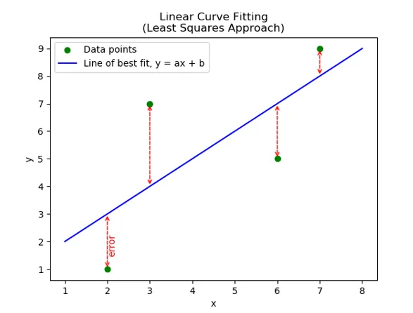
Let, there are data points (x1,y1); (x2, y2);...........(xn,yn) and assume the best fit for his curve as y=f(x). y=f(x) will be the best fit if the sum of the squares of errors is less.

Take point (Xi, Yi)

error=|y(i)-f(x(i))|

to remove the mod, we can square on both sides,

we get,

error^2=(y(i)-f(x(i)))^2

For n data points we get n errors and by adding ll these errors we get the sum of squares of all these errors(i.e, SSE).

If we differentiate this SSE with respect to coefficients of the polynomial. We get n no. of equations. By solving these equations we get the values of all the coefficients.

Procedure:

1. Linear polynomial is fitted to the given data and it's r square value are found through the following code-

import math
import numpy as np 
import matplotlib.pyplot as plt 
from scipy.optimize import curve_fit
import statistics

def f(x,a,b):
	return a*x+b

def read_file():
	temperature=[]
	cp=[]
	for line in open('data','r'):
		values=line.split(',')
		temperature.append(float(values[0]))
		cp.append(float(values[1]))

	return [temperature,cp]

#Main 
temperature, cp= read_file()
popt,pcov= curve_fit(f,temperature,cp)
fit_cp=f(np.array(temperature), *popt)

#plots
plt.plot(temperature,cp)
plt.plot(temperature, fit_cp)
plt.legend(['Actual data', 'Curve fit'])
plt.xlabel('Temperature')
plt.ylabel('cp')
plt.title('curve fitting')
plt.show()

#Rsquare value
sse=0
err=0
ssr=0
sst=0
for i in range(np.size(cp)):
	err=(cp[i]-fit_cp[i])
	sse=sse+pow(err,2)
	ssr=ssr+pow((fit_cp[i]-statistics.mean(cp)),2)
sst=sse+ssr
r_square=ssr/sst
print('R square value is:', r_square)

Code explanation-
A function is taken for the required linear polynomial function to be fitted to the given data. Another function is taken named read_file which reads the given 'data' file and returns the temperature and cp arrays. Fit parameters and covariance are found using the curve_fit command and these values are stored in popt and pcov respectively. Then, the corresponding values of f(x) are found for corresponding values of temperatures and corresponding fit coefficients. Plots are drawn for temperatures vs cp and temperatures vs fit_cp. r_square value is also found to know how well the curve has been fit.

2. Cubic polynomial is fitted to the given data and its r square value are found through the following code-

import math
import numpy as np 
import matplotlib.pyplot as plt 
from scipy.optimize import curve_fit
import statistics

def f(x,a,b,c,d):
	return a*pow(x,3)+b*pow(x,2)+c*x+d

def read_file():
	temperature=[]
	cp=[]
	for line in open('data','r'):
		values=line.split(',')
		temperature.append(float(values[0]))
		cp.append(float(values[1]))

	return [temperature,cp]

#Main 
temperature, cp= read_file()
popt,pcov= curve_fit(f,temperature,cp)
fit_cp=f(np.array(temperature), *popt)

#plots
plt.plot(temperature,cp)
plt.plot(temperature, fit_cp)
plt.legend(['Actual data', 'Curve fit'])
plt.xlabel('Temperature')
plt.ylabel('cp')
plt.title('curve fitting')
plt.show()

#Rsquare value
sse=0
err=0
ssr=0
sst=0
for i in range(np.size(cp)):
	err=(cp[i]-fit_cp[i])
	sse=sse+pow(err,2)
	ssr=ssr+pow((fit_cp[i]-statistics.mean(cp)),2)
sst=sse+ssr
r_square=ssr/sst
print('R square value is:', r_square)

Code explanation-
A function is taken for the required cubic polynomial function to be fitted to the given data. Another function is taken named read_file which reads the given 'data' file and returns the temperature and cp arrays. Fit parameters and covariance are found using the curve_fit command and these values are stored in popt and pcov respectively. Then, the corresponding values of f(x) are found for corresponding values of temperatures and corresponding fit coefficients. Plots are drawn for temperatures vs cp and temperatures vs fit_cp. r_square value is also found to know how well the curve has been fit.

3. In order to make the curve fit perfect, we can increase the order of the function. It can clearly be seen from the plots in the result that as the order of the curve to be fit is increased the curve fit is slowly approaching perfection.

Result:

Linear polynomial curve fit-

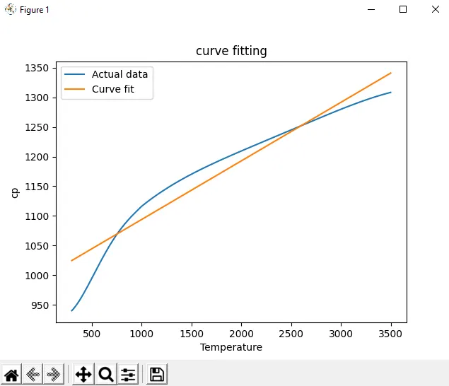
R square value for the linear curve fit -

Cubic polynomial curve fit-

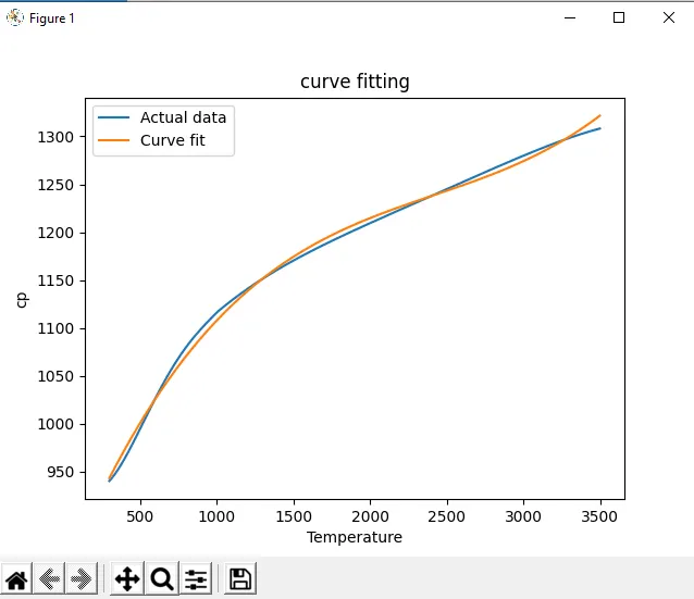
R square value for the cubic curve fit -

Conclusion:

The code is written to fit a linear and cubic polynomial for the Cp data. Results show that the cubic polynomial fit is better than the linear polynomial curve fit as the R square value for the polynomial curve fit is greater than that for linear polynomial curve fit.