Week 3 - Solving second order ODEs

Aim:

The main objective is to write a program that solves the following ODE. This ODE represents the equation of motion of a simple pendulum with damping for 0-20 sec, for angular displacement=0, angular velocity=3 rad/sec at time t=0.

Theory:

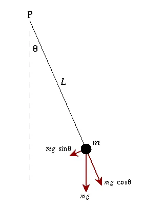
This is a simple pendulum that has a mass 'm', length 'L', and is under a damping phenomenon whose damping coefficient is 'b'. Equation of motion of a simple pendulum can be given by a 2nd order ODE, which is given as-

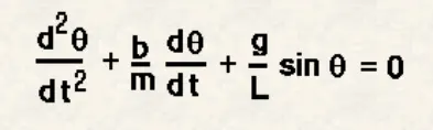
This is a 2nd order ODE. This ODE can be split into two 1st order ODE's. Among these two ODE's one describes velocity and the other acceleration.

The two 1st order ODE's obtained are, as follows-

These two 1st order ODE's can be solved to get theta1(i.e, displacement) and theta2(i.e, velocity) values.

Procedure:

1. Required values of damping coefficient, mass, acceleration due to gravity, and length of the pendulum are initialized.

2. The following python code is written for solving the given 2nd order ODE:

"""
solving of 2nd order ODE
"""

import math
import matplotlib.pyplot as plt
import numpy as np
from scipy.integrate import odeint

def solution_vector(theta_initial,t,b,g,l,m):
	theta1=theta_initial[0]
	theta2=theta_initial[1]
	theta1_dt=theta2
	theta2_dt=(-b/m)*theta2 - (g/l)*math.sin(theta1)
	theta_dt=[theta1_dt,theta2_dt]
	return theta_dt

b=0.05 #damping coefficient 
g=9.81 # accelaration due to gravity
l=1 # length of the pendulum in metres
m=1 # mass of the pendulum in kg's

#time points
t=np.linspace (0,20,200)

#initial condition
theta_initial=[0,5]

# solving of ODE
theta=odeint(solution_vector, theta_initial, t, args=(b,g,l,m))

#plots
plt.xlabel('time')
plt.ylabel('plot')
plt.legend()
plt.plot(t,theta[:,0], label='theta2')
plt.plot(t,theta[:,1], label='(-b/m)*theta2 - (g/l)*sin(theta1)')
plt.legend()
plt.show()

Code explanation-

The required methods like math, matplotlib.pyplot, numpy, and in scipy.integrate odeint are imported. Next, a function is defined called solution_vector, and in that function, theta1_dt and theta2_dt are being calculated and returned which are the components of the solution vector. The values such as damping coefficient, the mass of the pendulum, length of the pendulum, and acceleration due to gravity are initialized. Two hundred values between 0 to 20 are created and are stored in t(i.e, time). Initial values of distance and velocity are given. Then, using odeint command solution vectors is obtained and is stored in theta. Theta variable contains 2 columns and many rows. 1st column is displacement values and the 2nd column is velocity values. Then, we are plotting the plots for displacement vs time and velocity vs time.

3. An animation is also done to demonstrate the motion of the pendulum.

Error occurred during coding:

This error occurred because instead of passing the initial values of theta to the theta1, theta2 variables inside the function, I initialized theta[0] and theta[1] values to theta1 and theta2 variables, which are actually not defined, this is wrong. So I rectified this error by passing the correct values to the correct variables.

Result:

Plot obtained-

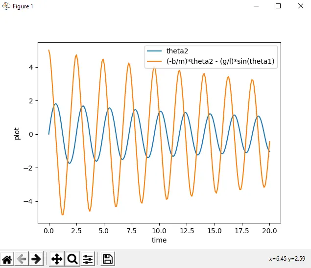
Animation of the simple pendulum-

The animation of the simple pendulum for the given values o f0-20 sec, for angular displacement=0, angular velocity=3 rad/sec at time t=0 can be seen through this link- https://www.youtube.com/watch?v=hP85Zj-3-R0

Conclusion-

A program solving the given 2nd order ODE is written and simulation of the simple pendulum can be seen through the given link given above.