Week 2 Air standard Cycle

Aim:

The aim of this project is to write a code that can solve an otto cycle and make plots for it. Main objectives of this project are:

1. Write a code to create a PV diagram

2. To find the output of the thermal efficiency of the engine.

Theory:

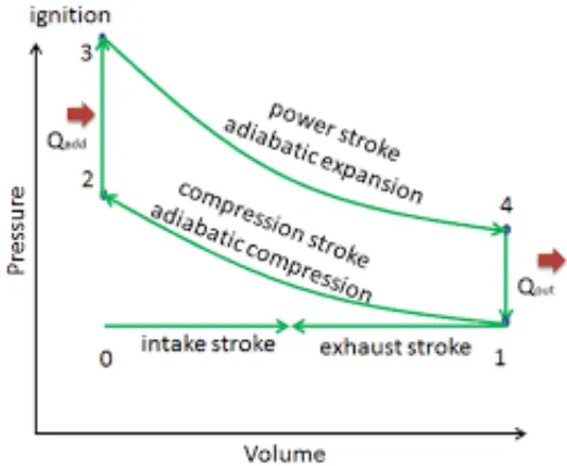
Otto cycle is a set of four processes - (1). 1-2: Adiabatic compression process, (2). 2-3: Isochoric heat addition process, (3). 3-4: Adiabatic expansion process, (4). Isochoric heat rejection process. For this cycle, the state variables are plotted on pressure vs volume plot.

1. 1-2, 3-4 processes are adiabatic processes. therefore it's an isentropic process. Isentropic processes follow the equation:

(p1*v1)^gamma= p2*v2^(gamma)

where,

gamma= Cp/Cv(i.e, ratio of specific heats)

p1,p2 are the pressure state variables defining the adiabatic process, and v1,v2 are the volume state variables defining the adiabatic process.

2. As the gas is considered as an ideal gas, the gas follows

p1*v1/t1=p2*v2/t2

where,

p1,p2 are the pressure state variables, and v1,v2 are the volume state variables, and t1, t2 are the temperature state variables.

3. Thermal efficiency of the Otto cycle is given by

thermal_efficiency= 1-(1/compression ratio^(gamma -1))

Procedure:

1. The temperature state variable at point 1 and point 3 be 500 and 1500. the corresponding value of pressure to point 1 temperature state variable be 101325 and take gamma(i.e, the ratio of specific heats as 1.4.

2. Take the bore as 0.1, stroke as 0.1, connecting rod length as 0.15, and compression ratio as 4.

3. Python code is written to plot the state variables and get a plot of otto cycle. The python code is as follows-

"""

Otto Cycle Simulator

"""
import math
import matplotlib.pyplot as plt
import numpy as np

def engine_kinematics(bore,stroke,con_rod,cr,crank_start,crank_end):
	a= stroke/2
	R= con_rod/a
	v_s= (math.pi/4)*pow(bore,2)*stroke
	v_c= v_s/(cr-1)
	theta= np.linspace(math.radians(crank_start),math.radians(crank_end),50)	
	v=[]
	for t in theta:
		term1=0.5*(cr-1)
		term2=R+1-math.cos(t)
		term3=pow(pow(R,2)-pow(math.sin(t),2),0.5)
		v.append((1+term1*(term2-term3))*v_c)
	return v
    	


#inputs
p1=101325
t1=500
t3=1500
gamma=1.4 # ratio of specific heats

#geometric dimensions of engie
bore=0.1
stroke=0.1
con_rod=0.15 # length of connecting rod
cr=4 # compression ratio
# thermal effeciency
therm_eff= 1-(1/pow(cr,gamma-1))
print('Thermal effeciency of this otto cycle is', therm_eff)

#volume calculation 
v_s= (math.pi/4)*pow(bore,2)*stroke # swept volume
v_c= v_s/(cr-1) # clearence volume

# State point 1
v1=v_s+v_c

# State point 2
v2=v_c
p2=p1*pow(v1,gamma)/pow(v2,gamma)
temp=p1*v1/t1
t2=p2*v2/temp

#adiabatic compression curve
volumes_compress=engine_kinematics(bore,stroke,con_rod,cr,180,0)
pressures_compress=[]
for v in volumes_compress:
	constant=p1*pow(v1,gamma)
	pressures_compress.append(constant/pow(v,gamma))



# State point 3
v3=v2 # constant volume process
temp=p2*v2/t2
p3=temp*t3/v3
 
# State point 4
v4=v1
p4=p3*pow(v3,gamma)/pow(v4,gamma)
temp=p3*v3/t3
t4=p4*v4/temp


#adiabatic expansion curve
volumes_expand=engine_kinematics(bore,stroke,con_rod,cr,0,180)
pressures_expand=[]
for v in volumes_expand:
	constant=p3*pow(v3,gamma)
	pressures_expand.append(constant/pow(v,gamma))


plt.figure()
plt.title('Otto cycle')
plt.xlabel('volume')
plt.ylabel('pressure')
plt.plot(volumes_compress,pressures_compress)
plt.plot([v2,v3],[p2,p3])
plt.plot([v1,v4],[p1,p4])
plt.plot(volumes_expand,pressures_expand)
plt.show()

Code explanation- Required methods such as math, matplotlib.pyplot, and numpy are imported. Then a function is created with the name engine_kinematics. This function is used to calculate the values of volume for different values of the crank angle. In this function crank pin radius(i.e, a) and R are the variables and the required formulas are used to find these values. we are also finding different values of volume for different crank angles using the for loop and linspace command in the function and all these values of the volume are stored in a null matrix v and this is returned when the function is called. After the creation of the function, the assumed state variables are initialized and the geometric dimensions of the engine are also initialized and required ideal gas characteristic equation and adiabatic process characteristic equations are used to find the state variables at all the points(i.e, point1, point2, point3, and point 4). First, for the adiabatic compression curve, the function is called with crank_start=180 and crank_end=0 to get the corresponding volume values at different crank angles descending from 180 to 0. Then these values of the volume are stored in a variable. These values of the volume are used to find the corresponding values of pressure. Secondly, for the adiabatic expansion curve, the function is called with crank_start=0 and crank_end=180 to get the corresponding volume values at different crank angles ascending from 0 to 180. Then these values of the volume are stored in a variable. These values of the volume are used to find the corresponding values of pressure. Now we have all the required state variables to plot the otto cycle. Using the plot commands the otto cycle is plotted.

Result:

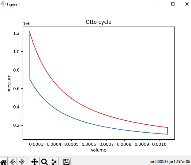
Otto cycle plot-

Thermal efficiency for this otto cycle is -

Conclusion:

PV plot was successfully plotted using the python code and the thermal efficiency of the otto cycle was also obtained from python.