Week 5 - Curve fitting

Objective(s):

Curve fitting using python.

Theory:

• Popt: It gives an array with values for the parameters used so that the sum of the squared remains of the data is minimized.
• Pcov: It is the array with the estimated covariance of the parameters in popt. It is used to calculate the standard deviation errors of popt.
• *in *popt stores the values of constant parameters, i.e. the constants a, b, c, d in the array popt.
• np.array(temperature) function stores the values of temperature in the form of array and passes it to the module function numpy.

Curve fitting is the process of constructing a curve, or mathematical functions, which possesses the closest proximity to the real series of data. By curve fitting, we can mathematically construct functional relationship between the observed dataset and parameter values etc. It is highly effective in the mathematical modelling of some natural processes.

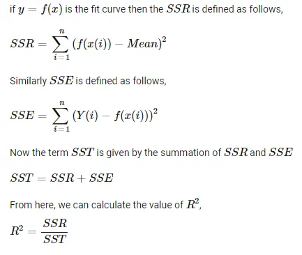
Sum of squares due to error(SSE),R-square,adjusted R-square, root mean squared error(RMSE) help us measure the goodness of fit.

R-square is the square of the correlation between the response values and the predicted responss values. Also called the square of multiple of the multiple correlation coefficient and the coefficient of multipe determination.

R²=`(SSR)/(SST)`

SSR= Sum of squares of regression.

Reference taken from the link mentioned in the video: Curve Fitting and criterion to choose best fit

Python Program:

#Curve fitting python program by Praharsh

import numpy as np
import matplotlib.pyplot as plt 
from scipy.optimize import curve_fit

##Curve fit for a linear equation


#Curve Fit function
def func_linear(t,a,b):
	return a*t+b

#reading thermodynamic data file (file is to be in the same folder as this program)
def read_file():
	temparature=[]
	cp=[]
	for line in open('data','r'):
		values= line.split(',')
		temparature.append(float(values[0]))
		cp.append(float(values[1]))
	return[temparature,cp]

#main program
temparature, cp=read_file()
popt , pcov=curve_fit(func_linear,temparature,cp)
fit_cp = func_linear(np.array(temparature),*popt)

#plotting using matplotlib
plt.plot(temparature,cp , color='blue',linewidth=3)
plt.plot(temparature,fit_cp,color='red',linewidth=3)
plt.title('Specific Heat Vs Temparature')
plt.legend(['Actual data','Curve fit'])
plt.xlabel('Temparature(K)')
plt.ylabel('Cp')
plt.show()

#R^2 value and RMSE value
mean_value=np.mean(cp)
error_linear= np.array(cp)-np.array(fit_cp)
error_sq_linear=np.square(error_linear)
sse_linear=sum(error_sq_linear)
ssr_linear=[x- mean_value for x in fit_cp ]
ssr_sq_linear=np.square(ssr_linear)
ssrr_linear=sum(ssr_sq_linear)
rsq_linear= 100*ssrr_linear/(ssrr_linear+sse_linear)
rmse_linear= pow((sse_linear/3200),0.5)
print('R^2:',rsq_linear)
print('RMSE:',rmse_linear)

##Curve fit for a quadratic equation

#Curve Fit function
def func_quadratic(t,a,b,c):
	return a*pow(t,2)+b*t+c

#reading thermodynamic data file (file is to be in the same folder as this program)
def read_file():
	temparature=[]
	cp=[]
	for line in open('data','r'):
		values= line.split(',')
		temparature.append(float(values[0]))
		cp.append(float(values[1]))
	return[temparature,cp]

#main program
temparature, cp=read_file()
popt , pcov=curve_fit(func_quadratic,temparature,cp)
fit_cp = func_quadratic(np.array(temparature),*popt)

plt.plot(temparature,cp , color='blue',linewidth=3)
plt.plot(temparature,fit_cp,color='red',linewidth=3)
plt.title('Specific Heat Vs Temparature')
plt.legend(['Actual data','Curve fit'])
plt.xlabel('Temparature(K)')
plt.ylabel('Cp')
plt.show()

#R^2 value and RMSE value
mean_value=np.mean(cp)
error_quadratic= np.array(cp)-np.array(fit_cp)
error_sq_quadratic=np.square(error_quadratic)
sse_quadratic=sum(error_sq_quadratic)
ssr_quadratic=[x- mean_value for x in fit_cp ]
ssr_sq_quadratic=np.square(ssr_quadratic)
ssrr_quadratic=sum(ssr_sq_quadratic)
rsq_quadratic= 100*ssrr_quadratic/(ssrr_quadratic+sse_quadratic)
rmse_quadratic= pow((sse_quadratic/3200),0.5)
print('R^2:',rsq_quadratic)
print('RMSE:',rmse_quadratic)
##Curve fit for a cubic equation

#Curve Fit function
def func_cubic(t,a,b,c,d):
	return a*pow(t,3)+b*pow(t,2)+c*t+d

#reading thermodynamic data file (file is to be in the same folder as this program)
def read_file():
	temparature=[]
	cp=[]
	for line in open('data','r'):
		values= line.split(',')
		temparature.append(float(values[0]))
		cp.append(float(values[1]))
	return[temparature,cp]

#main program
temparature, cp=read_file()
popt , pcov=curve_fit(func_cubic,temparature,cp)
fit_cp = func_cubic(np.array(temparature),*popt)

plt.plot(temparature,cp , color='blue',linewidth=3)
plt.plot(temparature,fit_cp,color='red',linewidth=3)
plt.title('Specific Heat Vs Temparature')
plt.legend(['Actual data','Curve fit'])
plt.xlabel('Temparature(K)')
plt.ylabel('Cp')
plt.show()

#R^2 value and RMSE value
mean_value=np.mean(cp)
error_cubic= np.array(cp)-np.array(fit_cp)
error_sq_cubic=np.square(error_cubic)
sse_cubic=sum(error_sq_cubic)
ssr_cubic=[x- mean_value for x in fit_cp ]
ssr_sq_cubic=np.square(ssr_cubic)
ssrr_cubic=sum(ssr_sq_cubic)
rsq_cubic= 100*ssrr_cubic/(ssrr_cubic+sse_cubic)
rmse_cubic= pow((sse_cubic/3200),0.5)
print('R^2:',rsq_cubic)
print('RMSE:',rmse_cubic)

Explanation of the code:

First math and matplotlib libraries were imported for mathematical calculations and plotting. Numpy library was imported to use for calculations on arrays. A linear, quadratic and cubic equation function was defined and data was calculated to plot according to them. Next a part of code was used to read the data file that was provided to extract the data from inside it. The data was then appended to empty arrays for temparature and cp. next curve_fit command was used to plot the curve by taking the two arrays for input data.Coefficient values and covariance of coefficients of the polynomials were stored in popt and pcov as arrays and stored. Next the data was used to plot the curve for all the three types of equations and the best fit was obtained by observation of the obtained graphs. R square values for all the three functions were calculated using the formulas given in theory. Then the graphs were displayed using show() command and r square values were printed.

Results:

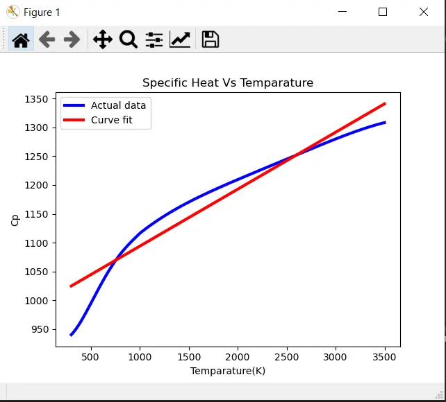
• Curve fit for linear equation

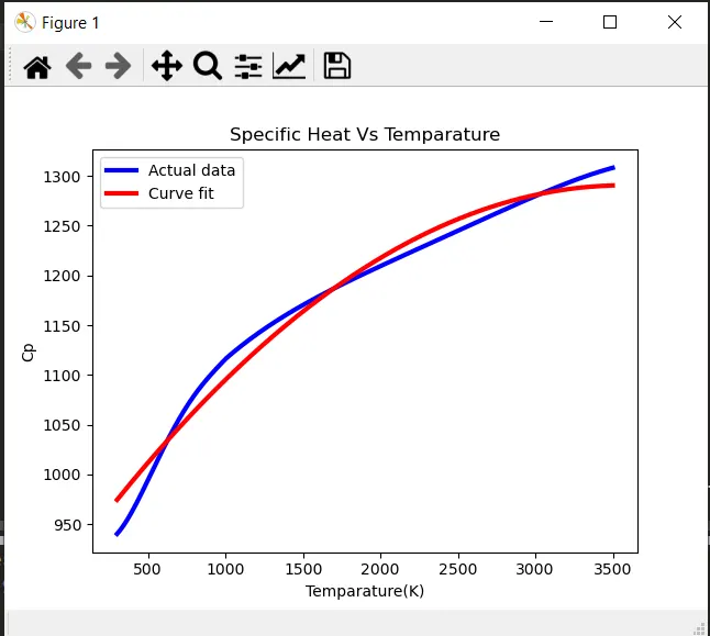
• Curve fit for quadratic polyomial

• Curve fit for cubic polynomial

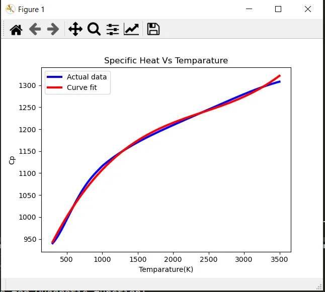
From the above graphs it is shown that the curve fits better when the degree of the equation/polynomial increases.

• Proof of program successful run

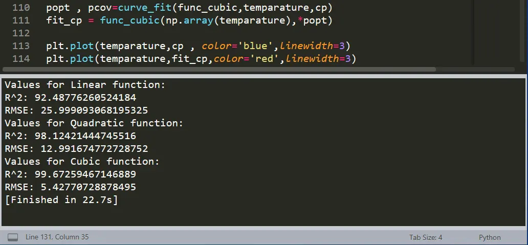
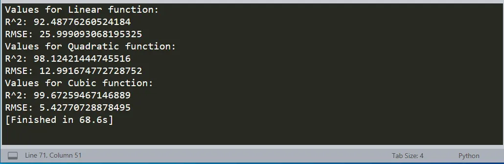
• R² Values

Conclusion:

The following were obtained as a result

• Best curve fit for the given data
• Execution time: 22.7 s