Week 3 - Solving second order ODEs

Objective(s):

To write a python program that will simulate the simple pendulum motion

Theory:

ODE is used to describe the transient behaviour of a system. A simple example is a pendulum

The way the pendulum moves depends on the Newtons second law. When this law is written down, we get a second order Ordinary Differential Equation that describes the position of the bob w.r.t time.

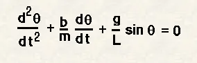
In the above equation,

g = gravity in m/s2,

L = length of the pendulum in m,

m = mass of the ball in kg,

b=damping coefficient.

Now we will convert/transform this second order ODE into first order ODE and then solve it to obtain the desired result.

Python Program:

#Pendulum Animation python program by Praharsh

#importing libraries
import numpy as np 
from scipy.integrate import odeint
import matplotlib.pyplot as plt
import math

#function that returns dz/dt
def model(theta,t,b,g,l,m):

	theta1= theta[0]
	theta2=theta[1]
	dtheta1_dt=theta2
	dtheta2_dt= -(b/m)*theta2-(g/l)*math.sin(theta1)
	dtheta_dt=[dtheta1_dt,dtheta2_dt]
	return dtheta_dt

#initialising values
b=0.05
g=9.81
l=1
m=1

#initial condition
theta_0=[0,3]

#time points
t=np.linspace(0,20,200)

#solve ode equation
theta= odeint(model,theta_0,t,args=(b,g,l,m))

#plot results 
plt.plot(t,theta[:,0],'b-',label=r'$\frac{d\theta_1}{dt}=\theta2$')
plt.plot(t,theta[:,1],'r--',label=r'$\frac{d\theta2}{dt}=-\frac{b}{m}\theta_2-\frac{g}{L}sin\theta_1$')
plt.ylabel('Plot')
plt.xlabel('Time')
plt.legend(loc='best')
plt.show()

#Pendulum Animation
ct=1
x0=5
y0=5
for i in range(len(t)):
	x1=x0+l*math.sin(theta[i,0])
	y1=y0-l*math.cos(theta[i,0])
	filename='pendulum' +str(ct)+ '.png'

	plt.figure()
	plt.plot([4,6],[5,5],'k-')
	plt.plot([x0,x1],[y0,y1])
	plt.plot(x1,y1,marker='o',markersize='10')
	plt.axis([3.5,6.5,3,6])
	plt.savefig(filename)
	ct=ct+1

Explanation of the code:

First, I’ve imported numpy, scipy, math, matplotlib libraries using the import command.

Now I defined a function where we will assume two theta variables theta1 and theta2. Theta2 is the first order differential equation of theta1 and theta2 is equal to theta.

After every calculation dtheta that was calculated was returned from the function. Then I’ve initialised b, g, l, m values to the values specified in the question. Initial conditions and time points were calculated and stored. odeint command was used to solve the ode equation.

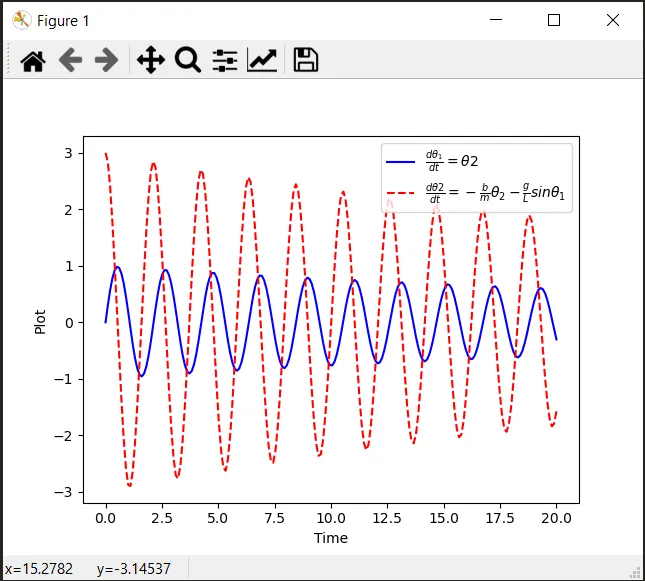
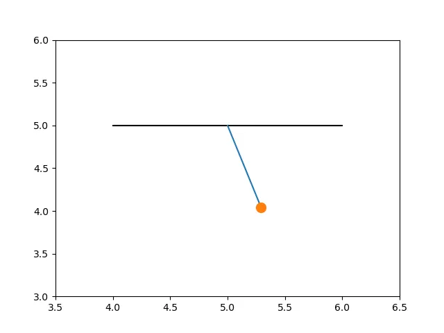
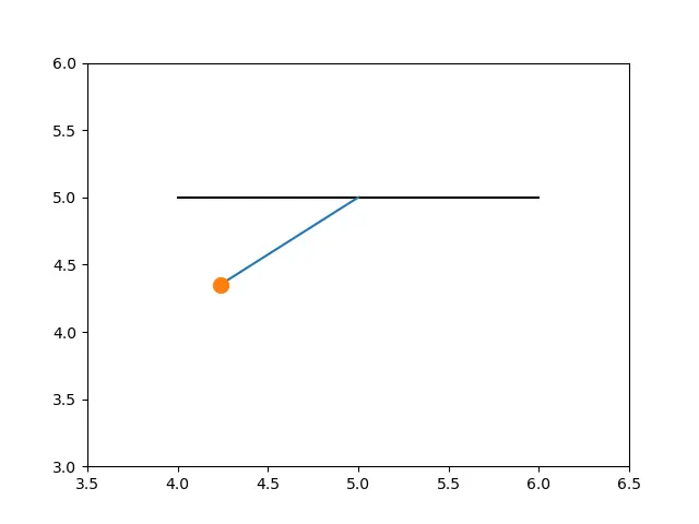
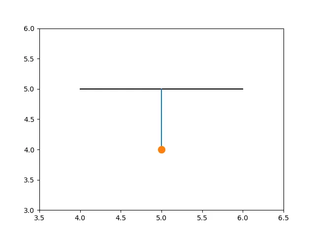
Then the points were plotted to obtain the graph as shown in results. Then for the animation part, for each value in time, I’ve created an image that represents the position of the pendulum. I’ve used the marker command to create a sphere at one end. One end of the pendulum is fixed and the other end moves according to the solution of the ODE obtained from the calculation.

Using a counter variable and saving picture at each calculation 200 images were obtained. Then the images were stitched to form an animation.

Errors made:

• Matplotlib library was imported but math library was forgotten to import
• Syntax errors were made
• Name errors were made

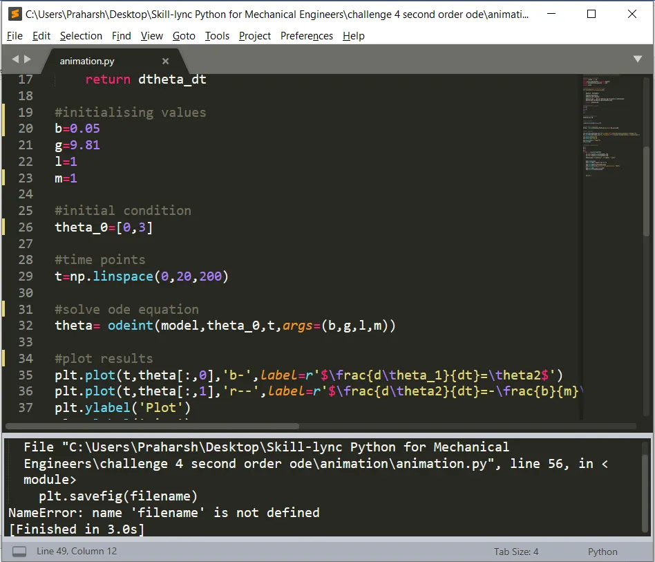
• Attribute errors were made

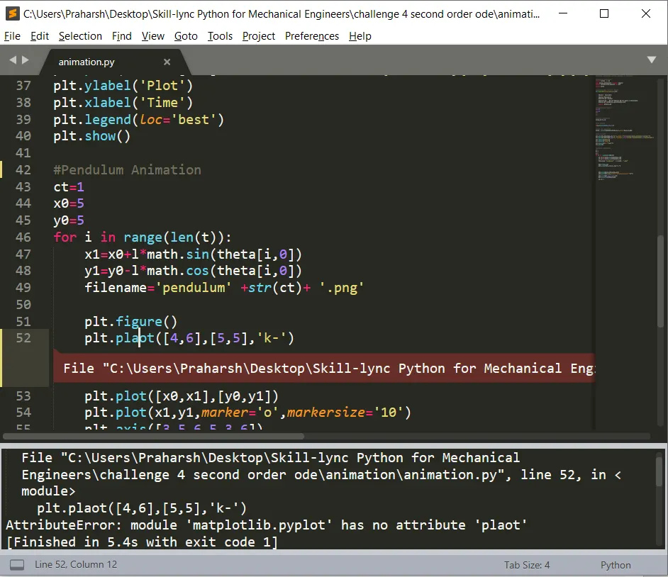
These errors were rectified by debugging the code at the end.

Result:

• Proof of program successful run

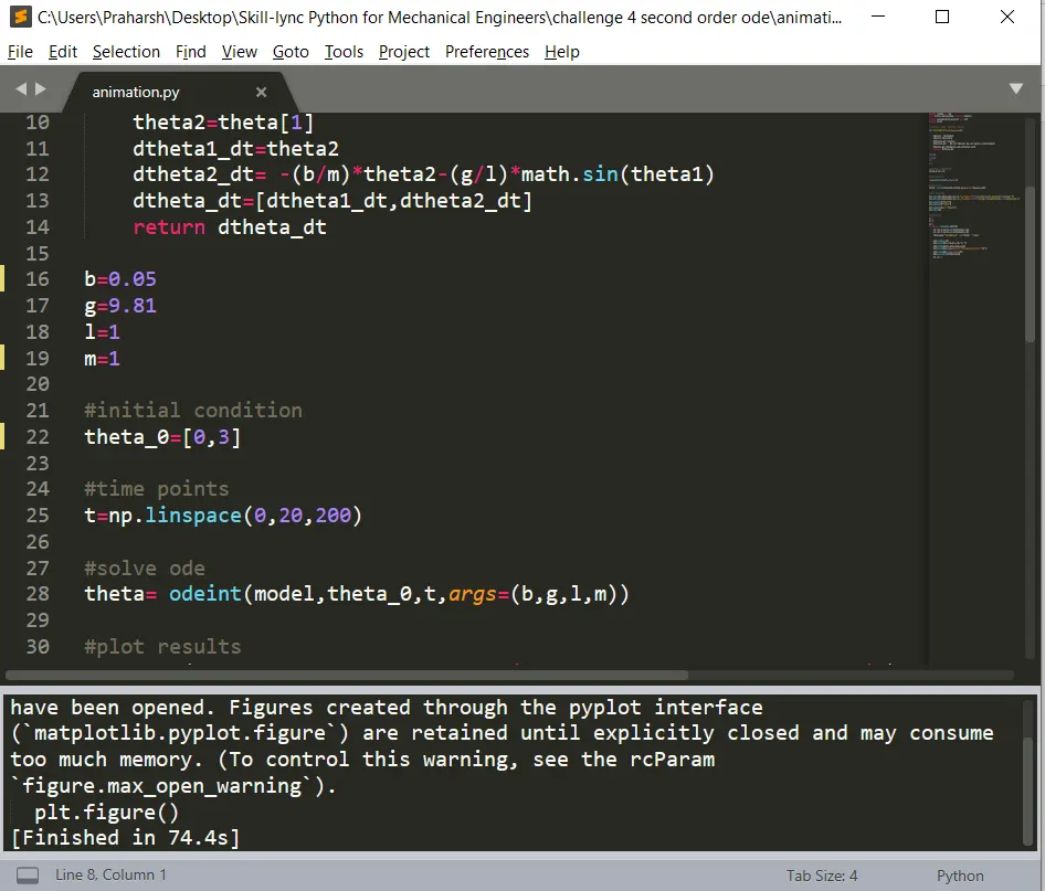
• Plot obtained.

• Sample image 1 for animation

• Sample image 2 for animation

• Animation

Conclusion: The following were obtained as a result

• Output plot of ODE
• Pendulum animation
• Execution time: 74.4 s

Drive link: https://drive.google.com/file/d/1ABPoTc1M_EQDgRIjeJ18Xhcfp04hjmMy/view?usp=sharing