Week 2 Air standard Cycle

Objective(s):

To write a python program

• To plot a P-V graph of otto cycle and study it.
• To calculate Thermal Efficiency.

Theory:

An Otto cycle is an idealized thermodynamic cycle that describes the functioning of a typical spark ignition piston engine. This cycle is most commonly found in automobile engines.

The Otto cycle is constructed from:

• Top and bottom of the loop: a pair of quasi-parallel and isentropic processes (frictionless, adiabatic reversible).
• Left and right sides of the loop: a pair of parallel isochoric processes (constant volume).

The processes involved in an otto cycle are as follows:

• Process 1 is an adiabatic (isentropic) compression of fuel air mixture as piston moves from BDC (Bottom dead centre) to TDC (Top dead centre)
• Process 2 is a constant volume heat transfer to the working gas from an external source (Spark from spark plug). This is burning of the charge at TDC
• Process 3 is an adiabatic (isentropic) expansion also called the power stroke
• Process 4 is a constant volume process in which heat is rejected when piston is at BDC (Exhaust stroke)

Formulas Used:

• PV^ɣ = Constant

Where, P=Pressure

V- Volume

ɣ= C_p/C_v  {C_p= specific heat of gas at constant pressure, C_v= specific heat of gas at constant volume}

• PV/T = Constant

Where, P= Pressure

V= Volume

T= Temparature

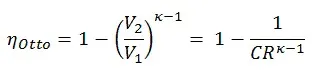
• Thermal Efficiency of otto cycle

• 

Python Program:

#otto cycle simulator python program by Praharsh

import math
import matplotlib.pyplot as plt


def engine_kinematics(bore,stroke,con_rod,cr,start_crank,end_crank):
	#geometric parameters
	a= stroke/2   #crankpin radius
	R= con_rod/a   #constant

	#volume parameters
	v_s=math.pi*(1/4)*pow(bore,2)*stroke
	v_c= v_s/(cr-1)

	sc = math.radians(start_crank)
	ec = math.radians(end_crank)

	num_values=50

	dtheta = (ec-sc)/(num_values-1)

	V=[]

	for i in range(0,num_values):
		theta=sc+i*dtheta
		term1= 0.5*(cr-1)
		term2= R+1-math.cos(theta)
		term3=pow(R,2) - pow(math.sin(theta),2)
		term3=pow(term3,0.5) 
		V.append((1+term1*(term2-term3))*v_c)
	return V
		
#inputs
p1=101325
t1=500
gamma=1.4
t3=2300

#geometric parameters
bore=0.1
stroke=0.1
con_rod=0.15
cr=8

#volume computaion
v_s= (math.pi/4)*pow(bore,2)*stroke
v_c=v_s/(cr-1)
v1= v_c+v_s

#state point 2
v2=v_c

#p2v2^gamma=p1v1^gamma
p2= p1*pow(v1,gamma)/pow(v2,gamma)


#p2v2/t2=p1v1/t1
rhs=p1*v1/t1
t2= p2*v2/rhs
V_compression=engine_kinematics(bore,stroke,con_rod,cr, 180,0)

constant= p1*pow(v1,gamma)

P_compression=[]

for v in V_compression:
	P_compression.append(constant/pow(v,gamma))
#state point 3
v3=v2

#p3v3/t3=p2v2/t2
rhs=p2*v2/t2
p3=rhs*t3/v3

V_expansion=engine_kinematics(bore,stroke,con_rod,cr, 0,180)

constant= p3*pow(v3,gamma)

P_expansion=[]

for v in V_expansion:
	P_expansion.append(constant/pow(v,gamma))

#state point 4
v4=v1

#p4v4^gamma= p3v3^gamma
p4=p3*pow(v3,gamma)/pow(v4,gamma)

#p4v4/t4=p3v3/t3
t4=p4*v4/rhs
#Thermal Efficiency
therm_eff= 1-(1/pow(cr,(gamma-1)))

plt.plot([v2,v3],[p2,p3])
plt.plot(V_compression,P_compression)
plt.plot(V_expansion,P_expansion)
plt.plot([v4,v1],[p4,p1])
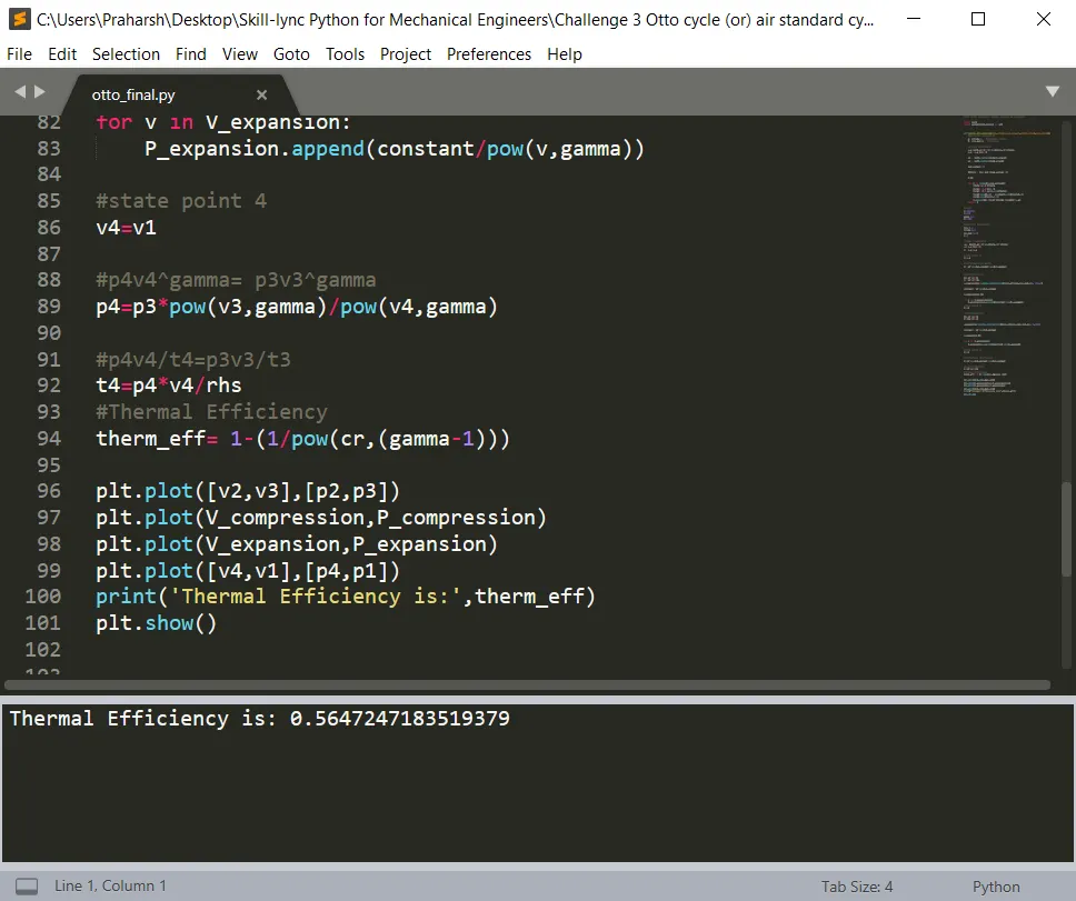
print('Thermal Efficiency is:',therm_eff)
plt.show()

Explanation of the code:

First, I’ve imported math and matplotlib library to use in the program. Then I’ve defined a function calculating velocities for different angles by randomly generating values of angle using a for loop between the start and end limits and stored them in an array. Then I’ve initialised few variables like bore, stroke, connecting rod length, crank pin radius, compression ratio etc.

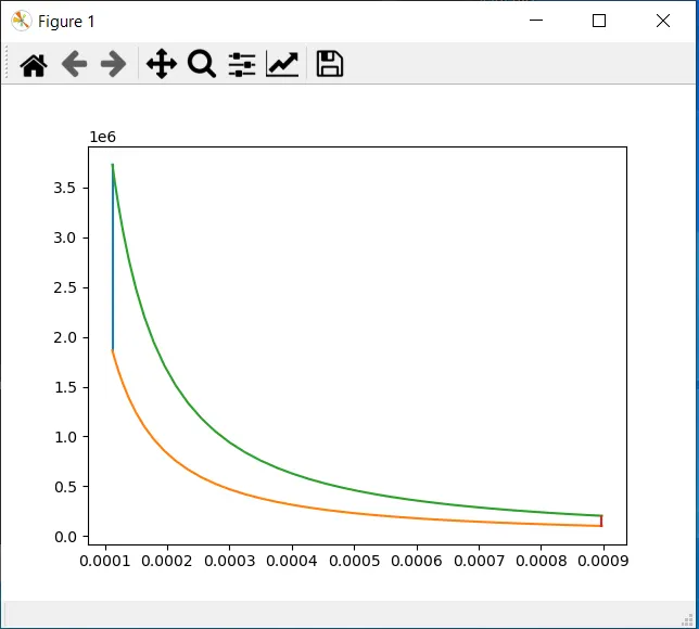
Then I’ve made calculations as per the formula given above and stored them in various variables. Once I calculated the states of different points using the formulae given, I have plotted the obtained values using matplotlib library. Then by using the show() command I obtained the graph of otto cycle.

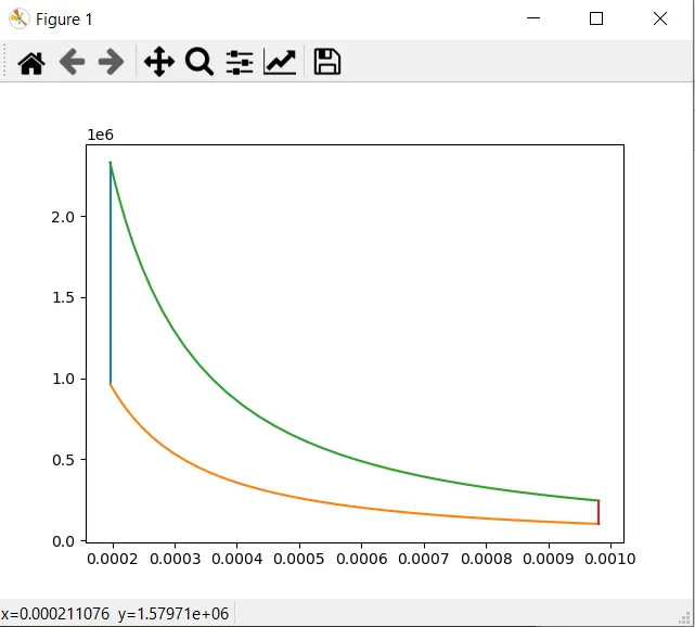
Then I changed the compression ratio and used different values, to check how the graph changes it’s shape under different compression ratios.

Result:

• Proof of program successful run and Thermal Efficiency of otto cycle

• Otto cycle graph( Compression ratio:8)

• Otto cycle graph( Compression ratio:5)

Conclusion: The following were obtained as a result

• P-V plot of Otto cycle
• Thermal Efficiency of otto cycle
• Execuation time: 2.7 s