Curve fitting with Python

Aim: To perform curve fitting with Python and obtain various parameters

Governing Equations:

The respective cubic and polynomial equations.

Explanation: Curve fitting is a vital process in many industries including product analysis, marketing, risk management, etc. If there is some data associated with a subject, we can plot graphs, fit a curve, and predict the future characteristics of the curve.

There are multiple types of curve fittings.

Linear Curve Fitting: In linear curve fitting, the data is fit in a straight line. However, the data need not be in a straight line. There is a high margin of error to this method, but the predictions can be made easily.

Polynomial Curve Fitting: Polynomial curve fitting is a bit more difficult to analyze than a linear curve fitting. However, accuracy is pretty high in this method.

Objectives: The main objectives of the project is being

1. To find what popt and pcov mean?
2. To identify the reason for using np.array(temperature)
3. To identify the use of the * in *popt mean?
4. To write a code to fit a linear and cubic polynomial for the Cp data.
5. To find a way in order to make the curve fit perfectly?
6. To Show empirically as to how well the curve has been fit.

The first step in the solution is to download the required data provided in the question. After downloading, we’ll have to place the data in the same folder as our code for easier access. Then we have to define a linear and a cubic polynomial as mentioned in the question.

We then have to process the data and make it workable with our code (the necessary operations such as separating, storing). Then, we can use the scipy library to make the required curve fit and plot them using matplotlib.

After plotting, we are checking the validity of our curve using the

Adjusted R-square, R-square (`R^2`), The sum of squares due to error (`SSE`), Root mean squared error (`RMSE`), The sum of squares due to error (`SSE`),

Body:

1. To find what popt and pcov mean?

The variables popt and pcov are used in the code to store the value returned by the curve fit. From reading the scipy docs, I found that popt is an array of optimal values for the parameters. pcov is a 2d array and is the estimated covarinace of popt.

2. The reason for using np.array(temperature)

np.array(temperature) converts all the

3. The use of the * in *popt

Since popt is an array, * is used to select all the values in the array.

4. Coding Language: Python 3.8.6 is used since the 3.9 version doesn’t yet have matplotlib support.

Code:

import numpy as np
from scipy.optimize import curve_fit
import math
import matplotlib.pyplot as plt

def func1(t, a, b):
    return a*t + b

def func2(t, a, b, c, d):
    return a*pow(t, 3) + b*pow(t, 2) + c*t + d

def read_file():
    temp =[]
    cp = []
    for line in open('data', 'r'):
        values = line.split(',')
        temp.append(float(values[0]))
        cp.append(float(values[1]))
    
    return [temp, cp]

temp, cp = read_file()
popt, pcov = curve_fit(func1, temp, cp)
popt2, pcov2 = curve_fit(func2, temp, cp)
fit_cp = func1(np.array(temp), *popt)
fit_cp1 = func2(np.array(temp), *popt2)

#plotting the curves

plt.plot(temp, cp, color= "blue", linewidth=3)
plt.plot(temp, fit_cp, color= "red", linewidth=3)
plt.xlabel('Temperature [K]')
plt.ylabel('Cp')
plt.legend(['Actual data', 'Linear Curve Fit'])
plt.savefig('Linearfit')
plt.show()
plt.clf()

plt.xlabel('Temperature [K]')
plt.ylabel('Cp')
plt.plot(temp, cp, color= "blue", linewidth=3)
plt.plot(temp, fit_cp1, color ="green", linewidth=3)
plt.legend(['Actual data', 'Cubic Curve Fit'])
plt.savefig('CubicFit')
plt.show()

plt.plot(temp, cp, color= "blue", linewidth=3)
plt.plot(temp, fit_cp1, color ="green", linewidth=3)
plt.plot(temp, fit_cp, color= "red", linewidth=3)
plt.legend(['Actual data', 'Cubic Curve Fit', 'Linear Curve Fit'])
plt.savefig('BothPlots')
plt.show()

#Curve Vaidity using the governing equations

#constants

numberofpts= np.size(cp)
total = np.sum(cp)
mean = total/numberofpts

#first curve

lsse = 0
lssr = 0

for i in range(numberofpts):
    lerr = abs((np.sum((cp[i] - fit_cp[i]))))
    lsse = lsse+pow(lerr,2)
    lssr = lssr+ np.sum(pow((fit_cp[i] - mean),2))

 
lsst = lsse + lssr
lrmse = pow((lsse/numberofpts),0.5)
lsqr = lssr/lsst

print('The SST for the Linear Curve Fit is :',lsst)
print('The RMSE for the Linear Curve Fit is  :',lrmse)
print('The R.Sq for the Linear Curve Fit is  :',lsqr)
print('------------------------------------------------------------------------------')


# Second Curve

csse = 0
cssr = 0

for j in range(numberofpts):
    cerr = abs(np.sum((cp[i] - fit_cp1[i])))
    csse = csse+(pow(cerr,2))
    cssr = cssr+np.sum(pow((fit_cp1[i] - mean),2))

 
csst = csse + cssr
crmse = pow((csse/numberofpts),0.5)
crsq= cssr/csst

print('The SST for the Cubic Curve Fit is :',csst)
print('The RMSE Value for the Cubic Curve Fit is:',crmse)
print('The R.Sq for the Cubic Curve Fit is :',crsq)

Code Explanation:

The required modules are imported in the first few lines. Then the linear and cubic equations are defined using functions as asked in the question. After that, a function is defined to read the data file provided in the problem statement. Since it is a comma-separated file, we are splitting each line at commas and storing the values in their respective arrays.

After this, the curve_fit function from the scipy module is called to give us a curve fit. The values returned by the function are stored in two arrays. The parameters are then passed to the function we defined earlier to obtain the curve.

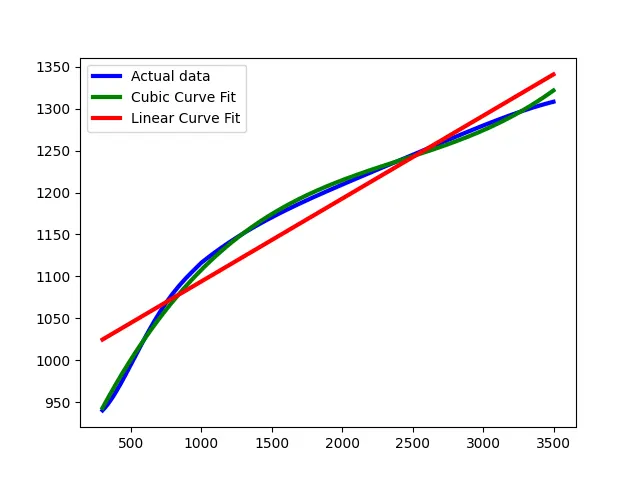
The curves are then plotted using matplotlib commands with all the legends, axes defined. We are storing these three plots in our local system for future reference.

Now, we are calculating the curve characteristics as per the governing equations. The Error, SSE, SSR, RMSE, SST, and R^2 are calculated for both the curves and are printed.

Output:

Results: (Also the 6th Objective)

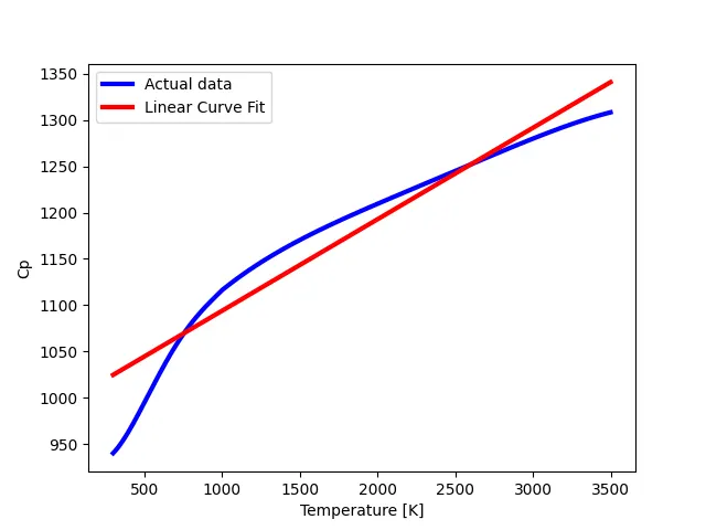
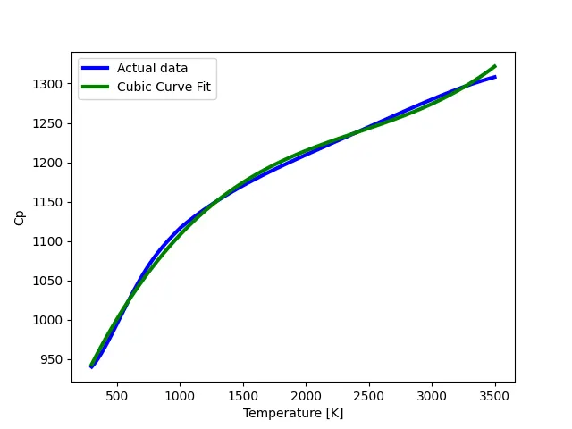
From the plots, it is clear that the linear curve is not the best fit for the given data. Meanwhile, the cubic curve is a decent fit. The values of the required parameters are also calculated in the output.

From the output, it is clear that the curves are a 92% fit. However, in the second case, the curves are 99.07% more alike. This conclusively proves that with an increase in the polynomial degree, the curves will resemble each other more.

We also know that the lower is the RMSE values, the better the curves fit. It is also clear from the RMSE values that the second curve is a better fit than the first curve.

The R square and the RMSE values suggest that the curves we obtained are good curves since there is a 90%+ resemblance for the linear curve and 99% for the cubic curve.

5. What to do to make the curves fit perfectly?

To make the curve fit perfectly, we should use a higher-order polynomial. It is clear from the above results that the higher is the polynomial's order, the better will be the fit.

let us just change the linear equation into a bi-qudratic equation.

def func1(t, a, b, c, d, e):
    return a*pow(t, 4) + b*pow(t, 3) + c*pow(t, 2) + d*t + e

Just changing function 1 and the word 'linear' to 'bi-quadratic' from the code in the 4th objective, we get the following outputs.

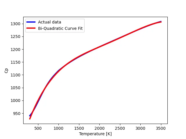
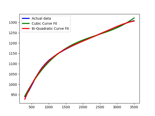
From the graphs and the R^2 and RMSE values, we can conclude that the higher-order polynomials fit the curve better.

Conclusion:

All the objectives are attained and the graphs are plotted.