Solving Ordinary Differential Equations using Python and Animating the Motion of a Simple Pendulum

Aim: To write a program that solves the following ODE. This ODE represents the equation of motion of a simple pendulum with damping

Governing Equations:

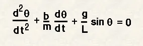
In the above equation,

b is the damping coefficient. No units

m = mass of the ball in kg,

g is the gravitational acceleration. Units m/s^2

L is the pendulum’s length

Equation Description: The governing equations is an ordinary differential equation of a simple pendulum. Using this equation, we can find the oscillations of the pendulum and make an animation for it.

Physics behind the equation: Damping is a prominent phenomenon in everyday life. Examples of damping include Springs, wall clocks, etc. In a pendulum, the bob’s position with respect to time can be given by an ODE.

Objectives: The main objective of the project is to write a program to simulate a simple pendulum’s motion.

Firstly, we have to get all the values required like the lengths, angle, mass, and the gravitational acceleration (constant) value Then, we have to use a programming language to solve the ODE and obtain the required plots. After this, we have to animate the pendulum’s motion as required in the problem using matplotlib.

Body:

Programming Language Used: Python 3.8.6 (since 3.9 doesn't yet have the matplotlib modules added)

Code:

import numpy as np
import math
from scipy.integrate import odeint
import matplotlib.pyplot as plt

#writing a function

def model(theta,t,b,g,l,m):
    
	theta1=theta[0]
	theta2=theta[1]
	dtheta1_dt=theta2
	dtheta2_dt=-(b/m)*theta2-(g/l)*math.sin(theta1)
	dtheta_dt=[dtheta1_dt,dtheta2_dt]
	return dtheta_dt

#input values

l=1
m=1
b=0.05
g=9.81

#init
theta_0=[0,3]

#time pnts
t=np.linspace(0,20,150)

#ODE Sol 
theta=odeint(model,theta_0,t,args=(b,g,l,m))

#plot results
plt.plot(t,theta[:,0],'b-',label=r'$frac{dtheta_1}{dt}=theta2$')
plt.plot(t,theta[:,1],'r--',label=r'$frac{dtheta2}{dt}=-frac{b}{m}theta_2-frac{g}{L}sintheta_1$')
plt.ylabel('plot')
plt.xlabel('time')
plt.legend(loc='best')
plt.show()

#anime
ctr=1
for theta in theta[:,0]:

	#fixed end of pendulum
	x0=0				
	y0=0

	x1=l*math.sin(theta)
	y1=-l*math.cos(theta)	

	plt.figure()

	plt.plot([-1,1],[0,0],"black",linewidth=5)
    
	plt.plot([x0,x1],[y0,y1],"red")
    
	plt.plot(x1,y1,'o',markersize=12)

	plt.xlim([-1,1])
	plt.ylim([-1.5,1])
	
	filename= str(ctr) + '.png'

	plt.savefig(filename)

	ctr+=1

Code Explanation:

In the first few lines, we are importing various modules that are required to run the program. Scipy is used to solve the ODE, matplotlib to plot the graphs, and Numpy to obtain values in a specific range.

After that, we described a model function that follows the governing principle. This function will be called later when solving the ODE. We are returning the final dtheta value back to the called variable. Initial conditions are then defined as per the requirement.

Then, we used the numpy attribute linspace to obtain 150 values in the range of (0,20). Now, we are using the odeint function and calling our previously defined function in it to combine both ODEs into one. The graphs are then plotted and labeled accordingly.

Various plots are obtained by changing the damping coefficient. You can find the obtained plots in the results section.

To produce the animation, we are taking the theta value in a range and finding the position of the pendulum at that angle. Using basic arithmetic, the positions are obtained and the graphs are plotted. To save the figures separately, a counter was initalized. After every image saved, the counter increases by 1.

Then I used an online Video maker to convert all the pictures into a video. The link to the youtube animation can be found below.

Results:

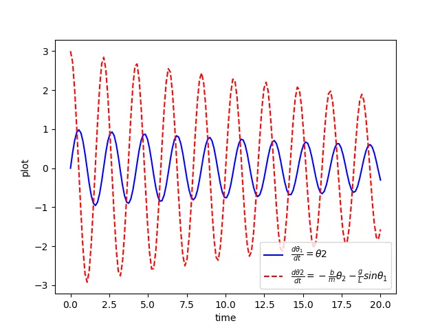
Damping coefficient 0.05

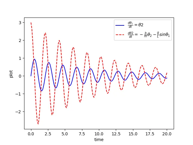
Damping Coefficient: 0.2

Motion of a Simple Pendulum Animation

Results:

We can observe the damping of the pendulum in the above plots. By changing the damping coefficient, we can determine how quickly a pendulum can come to rest (slow decrease in the angular velocity of the pendulum eventually brings it to rest. By increasing the damping coefficient, we are increasing the rate of decrease). From the animation, we can see the simple pendulum's motion which is just as expected.

Conclusion

The required plots are obtained and the animation was rendered.