Otto Cycle Solver Using Python

Aim: To write code that can solve an otto cycle and make plots for it, and find the Thermal efficiency of the Otto Cycle.

Governing Equations:

T2/T1 = (V1/V2)^(ɣ-1)

T3/T4 = (V4/V3)^(ɣ-1)

η% = 100*(1- (v2/v1)^(ɣ-1))

V/Vc = 1 + ½(rc - 1)[R + 1 - Cosθ - (R^2 - Sinθ^2)^½ ]

In the above equations,

T1, T2, T3, T4 are the temperatures at the end of each step in an otto cycle. Units - K

V1, V2, V3, and V4 are their corresponding volumes. Units - m^3

η is the efficiency of the Otto Cycle. No units

Ɣ is the ratio of specific heats. No units

rc is the compression ratio. No units

θ is the crank angle

Equation Description: The equations are used to derive the unknowns at the beginning and the end of each step. Only by knowing these values, will we be able to plot the graph.

Physics behind the equation:

In an Otto Cycle, there are four different steps taking place.

1. Air is drawn in at a constant pressure
2. Adiabatic Compression
3. Constant Volume Heat Transfer
4. Adiabatic Expansion

The governing equations are derived from the standard relations that can be applied to the above processes.

Objectives: The main objective of the project is to solve an otto cycle and make plots for it using Python.

Firstly, we have to get all the values required like the stroke length, crank angles, connecting rod lengths, initial temperatures and pressures, gamma, bore length, connecting rod lengths, etc. Then, we have to use relations to obtain the unknown quantities. Before drawing the graph we have to create a function to represent the volume change.

The function takes all the mentioned values and gives the volume values at different places in the process. We can use this information to get the pressure values as well. Now, we have to plot the cycle using Matplotlib.

Body:

Programming Language Used: Python 3.8.6 (since 3.9 doesn't yet have the matplotlib modules added)

import math
import matplotlib.pyplot as plt

def engine_kinematics(bore, stroke, connRod, convratio, start_crank, end_crank):
    
    a = stroke/2
    R = connRod/a
    V_s = math.pi*(1/4)*pow(bore, 2)*stroke
    V_c = V_s/(convratio-1)

    sc = math.radians(start_crank)
    ec = math.radians(end_crank)
    num_values = 10

    dtheta = (ec-sc)/(num_values-1)

    V= []

    for i in range(0, num_values):
        theta = sc + i*dtheta
        term1 = 0.5*(convratio-1)
        term2 = R + 1 - math.cos(theta)
        term3 = pow(R, 2) - pow(math.sin(theta), 2)
        term3 = pow(term3, 0.5)

        V.append((1 + term1*(term2 - term3))*V_c)
    
    return V

p1 = 10123
t1 = 500
t3 =1500
gamma = 1.4

#geometry

bore =0.1
stroke = 0.1
connRod = 0.15
convratio = 3

#volume comp
v_s = (math.pi/4)*pow(bore, 2)*stroke
v_c = v_s/(convratio -1)
v1 = v_c + v_s

#RHS Const
rhs = p1*v1/t1

#point 2
v2 = v_c
p2 = p1*pow(v1, gamma)/pow(v2, gamma)
t2 = p2*v2/rhs
V_Compression = engine_kinematics(bore, stroke, connRod, convratio, 180, 0)

constant = p1*pow(v1, gamma)

P_Compression = []

for v in V_Compression:
    P_Compression.append(constant/pow(v, gamma))

#point 3
v3 = v2
rhs = p2*v2/t2
p3 = rhs*t3/v3

V_Expansion = engine_kinematics(bore, stroke, connRod, convratio, 0, 180)

constant = p3*pow(v3, gamma)

P_Expansion = []

for v in V_Expansion:
    P_Expansion.append(constant/pow(v, gamma))

#point 4

v4 = v1
p4 = p3*pow(v3, gamma)/pow(v4, gamma)
t4 = p4*v4/rhs

engine_Efficiency = 1- pow((v2/v1), gamma-1)
engine_Efficiency = engine_Efficiency*100
print ('The Efficiency of this engine is ' + str(engine_Efficiency) + '%')

plt.plot([v2, v3], [p2, p3])
plt.plot(V_Compression, P_Compression)
plt.plot(V_Expansion, P_Expansion)
plt.plot([v4, v1], [p4, p1])
plt.xlabel('Volume')
plt.ylabel('Pressure')
plt.show()

Code Explanation:

First, we import the math and matplotlib modules to perform calculations and plot the graphs. In the next step, I wrote a function to calculate the volume at different parts of the process. This function will help us plot the non-linear variation of the volume better and more accurately.

The function takes bore, stroke, connecting rod lengths, compression ratio, start crank angle, and end crank angles as input. Then we take a specific number of iterations (10 in this case) and perform the iterations to obtain the Volume as per the governing equation.

Since we are going to get a set of values, we are initializing an empty array and are storing all the values inside the array by using the append function in Python.

Now, the main body starts. We first initialize various values necessary as mentioned in the process. After getting these values, we first calculate the parameters in stage 1. There on, using basic arithmetic, we get stages 2, 3, and 4 in a similar fashion.

At steps 2 and 3, where compression and expansion occur, we call the function we defined at the beginning with all the required values and reversed angles. Since it is a closed system, we know that p1v1 power gamma is constant. We calculate this constant and then the pressure values from the volume values.

We then append the values to an empty array for storing. A similar function call will be repeated for the expansion process as well. After all the calculations, we can finally plot the graphs using the plot attribute in matplotlib. For easier identification, I also labeled the axes in the graph.

Output:

Result:

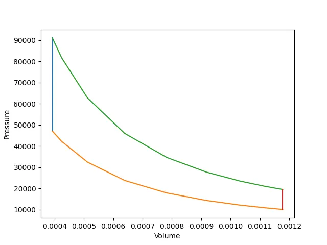
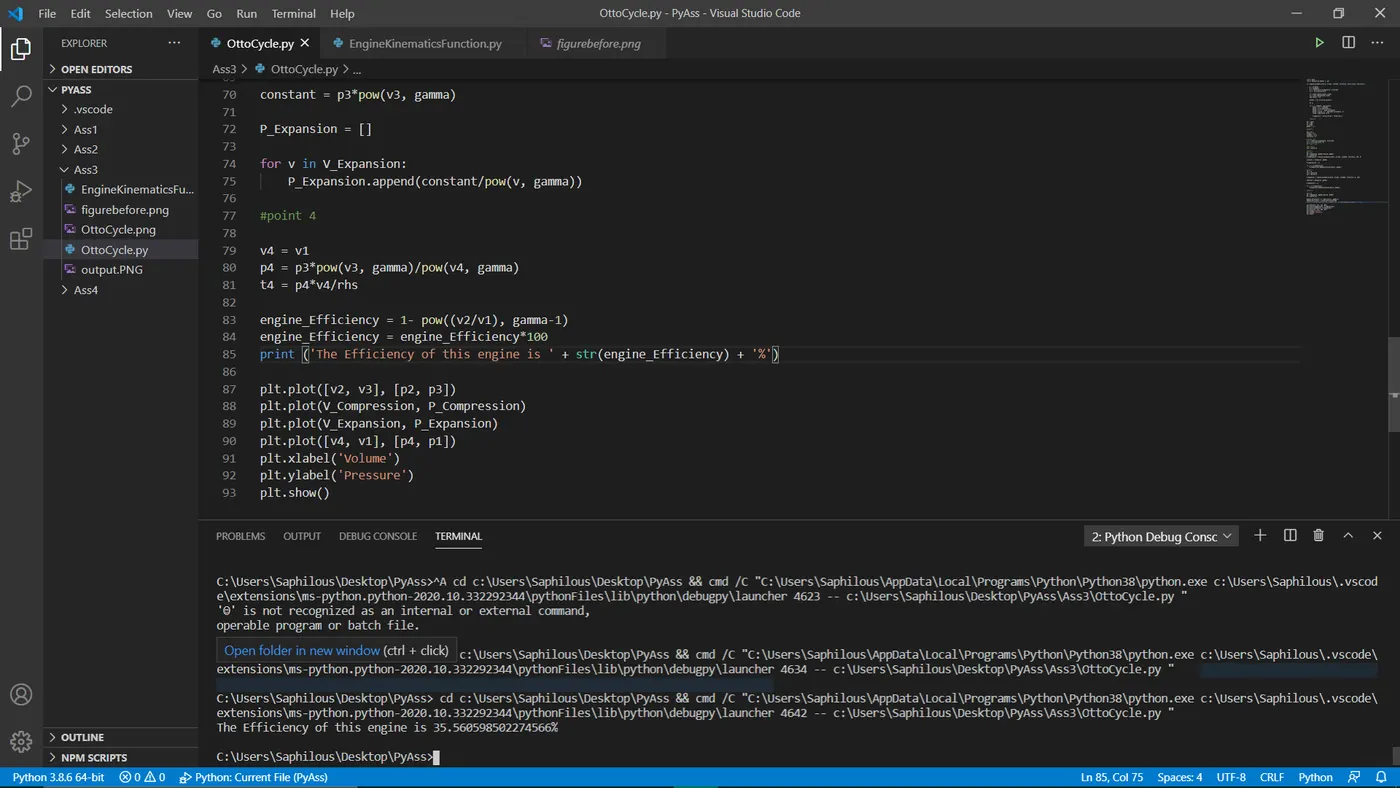
We obtained the Otto Cycle using matplotlib. The graph is as expected with an accurate representation of all the steps in the cycle. We also got the efficiency as shown in the above picture without much trouble. The vertical flat lines in the plot represent constant volume processes. The curved lines represent the adiabatic compression and expansion. By further decreasing the compression ratio, you can even get a smoother curve.

Conclusion:

A working Otto Cycle solver code is written that can also find the thermal efficiency.