Aim:- Write a program for curve fitting in python.

Theory:- Curve fitting is the way to make the mathematical model or create the curve that satisfies existing data at possible minimum error. In this challenge will be creating curve the satisfy the existing data of temperature (k) and specific enthalpy. It helps in data visualization. Curve fitting can use interpolation or smoothing for smooth fitting of data. By calculating error we can check which polynomial equation give best result.  Polynomial equations are used for curve fitting are -

1 First order polynomial
y=ax+b
2. Second order polynomial
Y= ax^2+bx+c
3. Third order polynomial
y= ax^3+bx^2+cx+d
and so on.
We shift towards higher degree of polynomial equation until get minimum error.

Procedure:-

1  Import matplotlib, math, numpy and curve fit.

2  Defining the function according to the degree of the polynomial equation.

3  defining read file, using for loop  take temperature and cp value in separate arrays

4  In the main program take data from the file, use popt to get the best estimates of data and pcov is covariance matrix showing the uncertainty and independence of each parameter in popt.

5 Using the curve fit make the curve with respect to the given temperature.

6 To check the accuracy of the result write code to get r square value if it will lie at 1 the fit will be the perfect fit and lies near 0.99 then the function will be good or best fit.

Code:-
1 First order polynomial equation
#Curve fitting by Rohit
# importing all required function

import math
import matplotlib.pyplot as plt
import numpy as np
from scipy.optimize import curve_fit

#fitting curve

def func(t ,a ,b ):
	return a*t+b

#Reading thermodynamic data file

def read_file():
	temperature=[]
	cp=[]
	for line in open ('data','r'):
		values=line.split(',')
		temperature.append(float(values[0]))
		cp.append(float(values[1]))
	return[temperature,cp]

# Main Program

temperature,cp=read_file()
popt, pcov = curve_fit(func,temperature,cp)
fit_cp= func(np.array(temperature),*popt)

# Calculating r_square value
n=len(temperature)
for i in range(n):
 error=cp-fit_cp
 sse=pow(error,2)
 rmse1=sse/6
 rmse=rmse1**0.5

 mean= np.array(cp[i])/np.array(i)
 ssr=(np.array(cp[i])-np.array(mean))**2
 sst=ssr+sse
 r_square=ssr/sst
 print(r_square)

# plotting graph for actual data and curve fit

plt.figure( 'First order equation')
plt.plot(temperature, cp, color='blue',linewidth=3)
plt.plot(temperature,fit_cp,color='red',linewidth=3)
plt.legend(['Actual data','Curve fit'])
plt.title('First order equation graph')
plt.xlabel('Temperature(k)')
plt.ylabel('Specific Heat')
plt.show()
2 Cubic polynomial Eqaution
#Curve fitting by Rohit
# importing all required function

import math
import matplotlib.pyplot as plt
import numpy as np
from scipy.optimize import curve_fit

#fitting curve

def func(t ,a ,b,c,d  ):
	return a*t**3+b*t**2+c*t+d

#Reading thermodynamic data file

def read_file():
	temperature=[]
	cp=[]
	for line in open ('data','r'):
		values=line.split(',')
		temperature.append(float(values[0]))
		cp.append(float(values[1]))
	return[temperature,cp]

# Main Program

temperature,cp=read_file()
popt, pcov = curve_fit(func,temperature,cp)
fit_cp= func(np.array(temperature),*popt)

# Calculating r_square value
n=len(temperature)
for i in range(n):
 error=cp-fit_cp
 sse=pow(error,2)
 rmse1=sse/6
 rmse=rmse1**0.5

 mean= np.array(cp[i])/np.array(i)
 ssr=(np.array(cp[i])-np.array(mean))**2
 sst=ssr+sse
 r_square=ssr/sst
 print(r_square)

# plotting graph for actual data and curve fit

plt.figure( 'Third order equation')
plt.plot(temperature, cp, color='blue',linewidth=3)
plt.plot(temperature,fit_cp,color='red',linewidth=3)
plt.legend(['Actual data','Curve fit'])
plt.title('Third order equation graph')
plt.xlabel('Temperature(k)')
plt.ylabel('Specific Heat')
plt.show()

Code Explanation:-

First import all the functions required for curve fitting. Using define function we define the equation to perform curve fitting for higher-order we can change the equation. To read the data and separate both the data we use for loop and make separate arrays. In the main program take data from the file, use popt to get the best estimates of data and pcov is covariance matrix showing the uncertainty and independence of each parameter in popt. Now to get the best fit only a graph is not enough, so calculating rms mean and r square is necessary.   r square approaching towards 1 is desired to get the best fit if it is exact 1 the fit will be the best fit. Now using function matplotlib Plotted the graph.
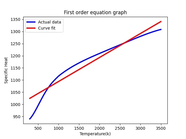
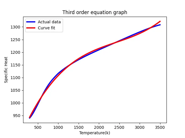
Results:- For 1st orde equation t square will lies between 0.96-0.99 and for 3rd order equation 0.999-0.9999 so it is clear that the 3rd order equation gives best fit as compared to 1 st order. So the third-order equation is approaching the existing original curve.

1.	What does popt and pcov mean?
Ans:-Popt is a dimensionless array that contains optimum values of parameters so that the square root of residual of function can be minimized.

Pcov is the estimated  covariance matrix of popt
2  What does np.array(temperature) do?

It is the array of all temperatures in the data arranged in sequence  in tuple form. In tuple we can not change the sequence or add values in the array .
3  What does the * in *popt mean?

It refers popt that contains all the constraint in it in the function.
4. Write code to fit a linear and cubic polynomial for the Cp data. Explain if your results are good or bad.
For linear and cubic polynomial the result is good but cubic is approaching towards perfect fit the R square is ranging 0.96-0.99 in linear and 0.999-0.9999 in the cubic polynomial.
5. What needs to be done in order to make the curve fit perfect?
The error should be considered to check fit is perfect or not. Always check at higher-order polynomial equation if R square value reached at 1 means the order of polynomial equation is perfect. If error is when increasing order of equation means we are going beyond perfect fit.
6.  Show empirically as to how well your curve has been fit.
From the output of the plotted graph by looking at R square value we can check that cubic fit is the best fit.