Aim:- Write a program to solves the ODE. This ODE represents the equation of motion of a simple pendulum with damping.

Theory:- ODE has many applications, one of them is to solve a simple pendulum equation. A simple pendulum has mass(bob ) at the end of the string another end is fixed on stationary support. The bob is hanging, when motion provided to the bob it oscillates with respect to the fixed end. If the damper is provided, at a certain period of time bob return at the initial condition, and the equation of motion is given by the following
                       (d^2 θ)/(dt^2 ) +(b/m)(dθ/dt)+(g/l)sinθ=0
Where
                   b= damping coefficient
                   m=mass of bob(kg)
                   g= acceleration due to gravity(m/s^2)
                   l= length(m)
                   θ= angle of the pendulum from y-axis
To solve this equation in python we have to convert it into one-degree equation, let us assume θ = θ1 now differentiate with respect to t, we get

                                     ( dθ)/dt=dθ1/dt1=θ2
Now new equation we get
                                     dθ2/dt2+(b/m) θ2+(g/l)sinθ1=0
Initial values are

m=1 kg
l=1m
b=0.05
g=9.81 (m/s^2)

At t=0
Angular displacement=0 rad
Angular Velocity= 3 rad/s

Procedures:-
1 First of all import matplotlib, math, scipy, numpy and odeint these functions will help to solve equations.

2. Now define all the parameters of a simple pendulum using the def function.

3. cover the 2-degree equation into 1-degree equation under the define function.

4. Provide all the initial data required to solve the equation.

5.Define initial parameters angular displacement and velocity at t=0 and upto 20 sec into 200 parts position of the bob will be considered.

6. Using odeint solve the equation at given parameters. The equation is solved for different angles and Odeint helps to solve the differential equation.

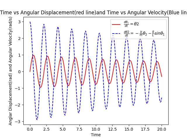
7. Now using outputs of the equation of angular displacement and angular velocity graph has been plotted.

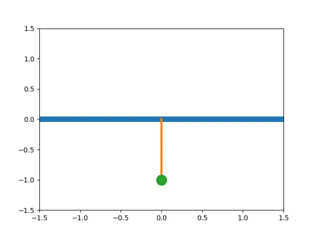
8. To make animation using the output data define the initial condition of string.

9. Now to get the position of the bob at different angles position of (x1,y1) have been calculated.

10.  The limiting condition for the graph is -1.5 and1.5 is considered.

11. Outputs of the images at different potion has been saved and with the help of image magic successfully animation has been created.

Code:-

# program to solve the Ordinary differential Equation of motion of simple pendulum
import numpy as np
import matplotlib.pyplot as plt
from scipy.integrate import odeint
import math
#function that returns dz/dt
def model(theta,t,b,g,l,m):
	theta1=theta[0]
	theta2=theta[1]
	dtheta1_dt=theta2
	dtheta2_dt=-(b/m)*theta2-(g/l)*math.sin(theta1)
	dtheta_dt=[dtheta1_dt,dtheta2_dt]
	return dtheta_dt

#Initial parameters(b(meter),g(m/s^2),l(m),m(kg))
b=0.05
g=9.81
l=1
m=1

#initial condition
theta_0=[0,3]

#time points
t=np.linspace(0,20,200)

#solve ode
theta=odeint(model,theta_0,t,args=(b,g,l,m))

#plot results
plt.plot(t,theta[:,0],'b-', label=r'$\frac{d\theta_1}{dt}=\theta2$',color='r')
plt.plot(t,theta[:,1] ,'r--', label=r'$\frac{d\theta2}{dt}=-\frac{b}{m}\theta_2-\frac{g}{L}sin\theta_1$',color='b')
plt.xlabel('Time')
plt.ylabel('Anglar Displacement(rad) and Angular Velocity(rad/s)')
plt.title('Time vs Angular Displacement(red line)and Time vs Angular Velocity(Blue line)')
plt.legend(loc='best')
plt.show()

# animation
# initial position of a simple pendulum
x0=0
y0=0
ct=1

for  i in theta[:,0]:
 # position of bob at differebt angles
  x1 =(l*math.sin(i))
  y1 = (-l*math.cos(i))
  file='test%05d.png'%ct
  ct=ct+1

  plt.figure()
  # plot graph  at the limit of -1.5 to 1.5 in both axis
  plt.plot([-1.5,1.5],[0,0],linewidth=8)
  plt.plot([x0,x1],[y0,y1],linewidth=3)
  plt.plot(x1,y1,'o',markersize=15)
  plt.xlim([-1.5,1.5])
  plt.ylim([-1.5,1.5])
  plt.savefig(file)

Code explanation:-
Imported all the required functions which will help to solve equations, mathematical expressions, and plot graph. Using def function define all the parameters inside this function, it can be used when there is need. Entered all the initial parameters and using linspace defined time range and solve the equation using odeint it helps to solve the differential equation. The graph has been plotted and using matplotlib all the essential parameters required to explain the graph have been given. Now to make animation using for loop calculated all the position of the bob at different angles has been created. Using image magic on the command prompt animation has been created.

Result:- Using all the input parameters simple pendulum motion for the given equation, the graph has been plotted and also using image magic animation has been created.
Aim:- Write a program to solves the ODE. This ODE represents the equation of motion of a simple pendulum with damping.

Theory:- ODE has many applications, one of them is to solve a simple pendulum equation. A simple pendulum has mass(bob ) at the end of the string another end is fixed on stationary support. The bob is hanging, when motion provided to the bob it oscillates with respect to the fixed end. If the damper is provided, at a certain period of time bob return at the initial condition, and the equation of motion is given by the following
                       (d^2 θ)/(dt^2 ) +(b/m)(dθ/dt)+(g/l)sinθ=0
Where
                   b= damping coefficient
                   m=mass of bob(kg)
                   g= acceleration due to gravity(m/s^2)
                   l= length(m)
                   θ= angle of the pendulum from y-axis
To solve this equation in python we have to convert it into one-degree equation, let us assume θ = θ1 now differentiate with respect to t, we get

                                     ( dθ)/dt=dθ1/dt1=θ2
Now new equation we get
                                     dθ2/dt2+(b/m) θ2+(g/l)sinθ1=0
Initial values are

m=1 kg
l=1m
b=0.05
g=9.81 (m/s^2)

At t=0
Angular displacement=0 rad
Angular Velocity= 3 rad/s

Procedures:-
1 First of all import matplotlib, math, scipy, numpy and odeint these functions will help to solve equations.

2. Now define all the parameters of a simple pendulum using the def function.

3. cover the 2-degree equation into 1-degree equation in the define function.

4. Provide all the initial data required to solve the equation.

5.Define initial parameters angular displacement and velocity at t=0 and upto 20 sec into 200 parts position of the bob will be considered.

6. Using odeint solve the equation at given parameters. The equation is solved for different angles and Odeint helps to solve the differential equation.

7. Now using outputs of the equation of angular displacement and angular velocity graph has been plotted.

8. To make animation using the output data define the initial condition of string.

9. Now to get the position of the bob at different angles position of (x1,y1) have been calculated.

10.  The limiting condition for the graph is -1.5 and1.5 is considered.

11. Outputs of the images at different potion has been saved and with the help of image magic successfully animation has been created.

Code:-

# program to solve the Ordinary differential Equation of motion of simple pendulum
import numpy as np
import matplotlib.pyplot as plt
from scipy.integrate import odeint
import math
#function that returns dz/dt
def model(theta,t,b,g,l,m):
	theta1=theta[0]
	theta2=theta[1]
	dtheta1_dt=theta2
	dtheta2_dt=-(b/m)*theta2-(g/l)*math.sin(theta1)
	dtheta_dt=[dtheta1_dt,dtheta2_dt]
	return dtheta_dt

#Initial parameters(b(meter),g(m/s^2),l(m),m(kg))
b=0.05
g=9.81
l=1
m=1

#initial condition
theta_0=[0,3]

#time points
t=np.linspace(0,20,200)

#solve ode
theta=odeint(model,theta_0,t,args=(b,g,l,m))

#plot results
plt.plot(t,theta[:,0],'b-', label=r'$\frac{d\theta_1}{dt}=\theta2$',color='r')
plt.plot(t,theta[:,1] ,'r--', label=r'$\frac{d\theta2}{dt}=-\frac{b}{m}\theta_2-\frac{g}{L}sin\theta_1$',color='b')
plt.xlabel('Time')
plt.ylabel('Anglar Displacement(rad) and Angular Velocity(rad/s)')
plt.title('Time vs Angular Displacement(red line)and Time vs Angular Velocity(Blue line)')
plt.legend(loc='best')
plt.show()

# animation
# initial position of a simple pendulum
x0=0
y0=0
ct=1

for  i in theta[:,0]:
 # position of bob at differebt angles
  x1 =(l*math.sin(i))
  y1 = (-l*math.cos(i))
  file='test%05d.png'%ct
  ct=ct+1

  plt.figure()
  # plot graph  at the limit of -1.5 to 1.5 in both axis
  plt.plot([-1.5,1.5],[0,0],linewidth=8)
  plt.plot([x0,x1],[y0,y1],linewidth=3)
  plt.plot(x1,y1,'o',markersize=15)
  plt.xlim([-1.5,1.5])
  plt.ylim([-1.5,1.5])
  plt.savefig(file)

Code explanation:-
Imported all the required functions which will help to solve equations, mathematical expressions, and plot graph. Using def function define all the parameters inside this function, it can be used when there is need. Entered all the initial parameters and using linspace defined time range and solve the equation using odeint it helps to solve the differential equation. The graph has been plotted and using matplotlib all the essential parameters required to explain the graph have been given. Now to make animation using for loop calculated all the position of the bob at different angles has been created. Using image magic on the command prompt animation has been created.

Result:- Using all the input parameters simple pendulum graph has been plotted for the given equation and also using image magic animation has been created.