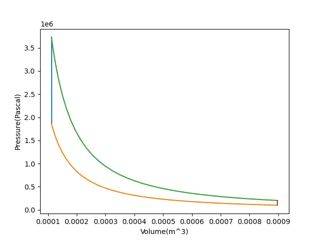
 Aim- Write code for the Otto cycle to calculate efficiency and plot PV graph using forward kinematics concepts.

Theory:- Otto cycle is nothing but a petrol engine cycle that is being used nowadays. This cycle consists of 4 processes to get power from petrol. Following are the processes-

1.Isentropic compression(process 1-2)
There is no heat transfer during compression.
2.Isochoric heat addition(process 2-3)
In this process heat addition occues at constant volume.
3.Isentropic expansion(process 3-4)
Ideally no heat transfer between system and surrounding only expansion occurs.
4.Isochoric heat rejection(process 4-1)
Heat rejection occurs at constant volume

By these 4 processes we get mechanical power and output power is used to drive the desire machine or mechanism. To calculate the efficiency of the Otto cycle following relation is given-
                             η =1-(1/(cr^(gamma-1)))

Where                     gamma=1.4 (for air)

          Compression ratio(cr)= (Total cylinder volume)/(clearance volume)

          Total cylinder volume=swept volume + clearance volume

                   Swept volume= (π/4)*d^2*l (m3)

               Clearance volume=(swept volume(m^3))/(compression ratio-1)

                            d = cylinder inner diameter(m)

                             l= stroke length(m)

To define the point of the PV graph we need some coordinates, so assuming air is following the ideal gas equation and conditions at the different point are as follows-
There are 4 points we get and conditions for points are pressure-volume and temperature are (P1,V1,T1),(P2,V2,T2),(P3,V3,T3) and (P4,V4,T4).
As we discussed the air follows ideal gas equation-
                                      PV=RT
At isentropic condition(Process 1-2) and ( Process 3-4)

                          (T1/T2)= (V2/V1)^(gamma-1) =(P1/P2)^((gamma-1)/gamma)

           and           (T3/T4) =(V4/V3)^(gamma-1) =(P3/P4)^((gamma-1)/gamma)
At isochoric condition(2-3) and(4-1)
                              V2=V3 and V4=V1
Now to get curvy nature of grapg we needs to have one relation

             V/Vc=[1+(1/2)(cr-1)+[R+1-cosθ-(R^2-(sinθ)^2)^(1/2)]

Where          a= stroke/2 (m)

               R= connecting rod length(m)/a
Where   θ is crank rotation angle and a= crank length(m).

Initial inputs are as follows

Initial pressure (P1)=101325 pascal
Initial Temperature= 500k
Maximum temperature=2300k

The geometric parameters are
Bore diameter=0.1 m
Length of stroke=0.1 m
Connecting rod lrngth= 0.15 m
Compression ratio= 8

Procedures-

1.First of all import math and matplotlib which will help to solve mathematical relations and plot the PV graph.

2.  Now enter the input parameters initial pressure, initial and maximum temperatures, and geometric specifications.

3. Provided formula to calculate initial volume by using input data also pressure and volume at point 2.

4. Using the relation of displacement of piston calculated the path of the piston at different angles of a crank between 180 to 0 degrees.

5.  By append arrange all the volume at different angles and using volume calculated pressure at various points.

6. At Process 2-3 and 4-1are isochoric process so volume will remain the same i.e v2=V3 and V1=V4.

7. Using the same relation by just change rotation angel 0 to 180 again calculate volume at various angles using the relationship among crank angles, crank length, and connecting rod length it will give change in the volume of the piston during the returning of stroke i.e. expansion process.

8. Provide code to calculate the pressure at different volumes and arrange it using append.

9. To calculate the efficiency of the engine wrote code of formula using compression ratio.

10. Now plot graph using all the data of volume and pressure.

Code:-

#Otto cycle PV plot and efficiency calculation
import math
import matplotlib.pyplot as plt
def engine_kinematics(bore,sroke,cod_rod,cr,start_crank,end_crank):
# engine kinematics
# geometry parameters
   a=stroke/2
   R=con_rod/a

   #volume parameters
   v_s=math.pi*(1/4)*(bore**2)*stroke
   v_c=v_s/(cr-1)

   sc=math.radians(start_crank)
   ec=math.radians(end_crank)
   num_value=50
   dtheta=(ec-sc)/(num_value-1)

   v=[]
   for i in range(0, num_value):
   	theta=sc+i*dtheta
   	term1=0.5*(cr-1)
   	term2=R+1-math.cos(theta)
   	term3=(R**2)-(math.sin(theta)**2)
   	term3=(term3**0.5)
   	v.append((1+term1*(term2-term3))*v_c)
   return v
#inputs
p1=101325
t1=500
gamma=1.4
t3=2300

#geometric parameters(bore, stroke ,connecting rod,compression ratio)
bore=0.1
stroke=0.1
con_rod=0.15
cr=8

#volume computation
#State point1
v_s=(math.pi/4)*(bore**2)*stroke
v_c=v_s/(cr-1)
v1=v_s+v_c


#state point2
v2=v_c

#p2v2^gamma=p1v1^gamma
p2=p1*(v1**gamma)/(v2**gamma)

#p2v2/t2 =p1v1/t1=rhs |t2=p2v2/rhs
rhs=p1*v1/t1
t2=p2*v2/rhs
v_compression=engine_kinematics(bore,stroke,con_rod,cr,180,0)
constant=p1*(v1**gamma)

p_compression=[]
for v in v_compression:
	p_compression.append(constant/(v**gamma))

# state point3
v3=v2

#p3v3/t3=p2v2t2=rhs
rhs=p2*v2/t2
p3=rhs*t3/v3
v_expansion=engine_kinematics(bore,stroke,con_rod,cr,0,180)

constant=p3*(v3**gamma)
p_expansion=[]
for v in v_expansion:
	p_expansion.append(constant/(v**gamma))

#state point4
v4=v1

#p4v4/t4=p3v3/t3=rhs
p4=p3*(v3**gamma)/(v4**gamma)

#otto cycle efficiency
gamma1=gamma-1

term4= pow(cr,gamma1)
efficiency=(1-(1/term4))*100


print('Efficiency =',efficiency)


plt.plot([v2,v3],[p2,p3])
plt.plot(v_compression,p_compression)
plt.plot(v_expansion,p_expansion)
plt.plot([v4,v1],[p4,p1])
plt.xlabel('Volume(m^3)')
plt.ylabel('Pressure(Pascal)')
plt.show()

Code explanation:-
First import math to use mathematical relations and matplotlib to plot the PV graph. Now using user define function put all the parameters required to calculate the volume. Now write code that will give the relationship among inputs and required to calculate volume at different points. Using for loop makes an array of volume that will iterate the function at the required number of times. Now enter all the inputs and geometrical parameters related to the piston cylinder. Recall define the function and calculate all the volumes between 180 to 0-degree angles and using these values by using for loop calculate pressure corresponding to volume and arrange in an array with the help of append. The pressure and volume at the different angles are calculated for the compression process now follow the same procedure only needs to change angles 0 to 180-degree volumes and corresponding pressure can be calculated. To calculate efficiency of the engine code of formula has been written for the ideal condition it depends on compression ration and gamma(i.e. 1.4 for air). With the help of matplotlib PV graph has been plotted and efficiency also calculated. Using print command value printed and using plt.show() graph comes on screen. We can see it on the screen.

Results:- By using all the input parameters and geometric parameters graph has been plotted and efficiency has been calculated. The efficiency of the engine is 56.47% in ideal condition.