Week 5.2 - Literature review: ODE Stability

OBJECTIVE:

The main objective is to study about ODE and writing a program in python to validate the results. After simulation we will get an idea about conditions required to get a stable solution.

THEORY:

An ordinary differential equation (ODE) is an equation that involves some ordinary derivatives of a function. Often, our goal is to solve an ODE, i.e., determine what function or functions satisfy the equation.

For example, let y be a dependent variable and x an independent variable, and y = f(x) is an unknown function of x. The notation for differentiation is dy/dx.

`(dy/dx) = x^2 + 2x+3`

`y(x) = 2x+2`

The above example is very easy to solve analytically, but when it comes to engineering problems, it is very difficult to solve the problems derivated with respect to time. So to overcome this problems, will use some numerical techniques to approximate the solution. Numerical integration is the backbone of all simulation tools. Understanding the basics of these methods can help a lot in interpreting the results. Bad or unexpected performance of such a method can be a hint to modeling errors and can motivate either the choice of another method or a modification of the model at hand.

Before going into the choice of methods used to simuate the solution, we need to know about the strability criteria of an ODE. Physical stability of an equilibrium solution to a system of differential equations addresses the behavior of solutions that start nearby the equilibrium solution. However, we will solve x˙ = f(x) using some numerical method. It is important that the approximations generated by the method are themselves close to the true solution. The concept of closeness in this context is referred to as numerical stability.

All ODE's are solved numerically using computer programs with different numerical schemes in which solved by explicit or implicit schemes. When in a function the dependent variable is not explicitly isolated on either side of the equation then the function becomes an implicit function. Whereas an explicit function is one which is given in terms of the independent variable.

Let us consider a simple ODE to perform simualtion and understand the stability concept,

`(dy/dx) = -1000y-e^-t`

For explicit function, we will use a forward differencing scheme, As we know Explicit scheme uses independant variables on RHS, the y value is known.

`(y^(n+1) -y^n)/(deltat) = -k*y^n - e^-t`

`y^(n+1) = y^n - k*y^n*deltat-e^-t*deltat`

Where, y^(n+1) is the new value updating from the previous time step y^n.

For Implicit function, we will use a backward differencing scheme, as we know the implicit scheme uses dependanr variables of a coupled equation which is solved by using iteravtive technique,

`(y^n -y^(n-1))/(deltat) = -k*y^n - e^-t`

`y^n = -k*y^n*deltat - e^(-t)*deltat+y^(n-1)`

Rearranging the equation,

`y^n= (y^(n-1)- e^-t*deltat)/(1+k*deltat)`

Where, y^n is the updated value solved by using the previous value of y^(n-1).

CODE SNIPPET:

"""
ODE stability literature review
Comparing the results of Explict and Implicit solutions with analytical solution.

dy/dt = -1000y - e^-t
Analytical solution: y(t) = (e^-1000t(1-e^999t))/999
Explicit solution: y(new) = y(old)- k*y(old)*dt - e^-t*dt
Implicit solution: y(new) = (y(old)-e^-t*dt)/(1+k*dt)

"""
import numpy as np 
import matplotlib.pyplot as plt 

t_start = 0		#simulation start time
t_end = 0.1		#simulation end time
dt = 2e-3		#time step
k = 1000		#constant value

#Defining the function for explicit scheme
def explicit_euler(t_end,dt):
	t = np.arange(0,t_end,dt)		#Creating a array for time 
	y = np.zeros(len(t))			# Creating an array for y

	#Creating a for loop for iterating the solution
	for i in range(1,len(t)):
		y[i] = y[i-1] + dt*(-k*y[i-1]-np.exp(-t[i-1]))
	return [t,y]

#Defining the function for implicit scheme
def implicit_euler(t_end,dt):
	t = np.arange(0,t_end,dt)		#Creating a array for time 
	y = np.zeros(len(t))			# Creating an array for y

	#Creating a for loop for iterating the solution
	for i in range(1,len(t)):
		y[i] = (y[i-1] - np.exp(-t[i-1])*dt)/(1+k*dt)
	return [t,y]

def analytical_solution(t_end,dt):
	t = np.arange(0,t_end,dt)
	y = np.zeros(len(t))

	for i in range(1,len(t)):

		y[i] = (np.exp(-k*t[i])*(1-np.exp((k-1)*t[i])))/(k-1)

	return[t,y]

#Returning the solution array from the function
t,y_explicit = explicit_euler(t_end,dt)
t,y_implicit = implicit_euler(t_end,dt)
t,y_analy = analytical_solution(t_end,dt)
plt.plot(t,y_explicit,'--',color='blue')
plt.plot(t,y_implicit,color='red')
plt.plot(t,y_analy,'-.',color='black')
plt.xlabel('time')
plt.ylabel('y')
plt.legend(['Explicit','Implicit','Analytical'])
plt.title('Variation of y with respect to time\n @ t = 0.1, dt = 2e-3, k = 1000')
plt.show()

PROCEDURE:

• Creating a function for both explicit and impicit schemes with an input of t_end and dt and returning the results array with [t,y]
• Using a for loop iterating the function near to solution.
• From wolframalpha, getting the analytical solution and as above creating the function.
• PLotting the results.

RESULTS:

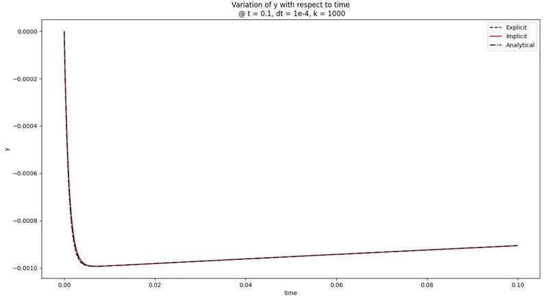
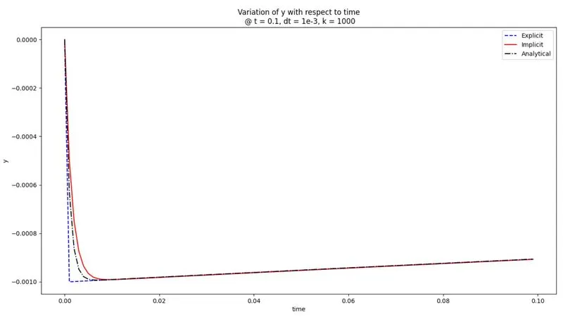
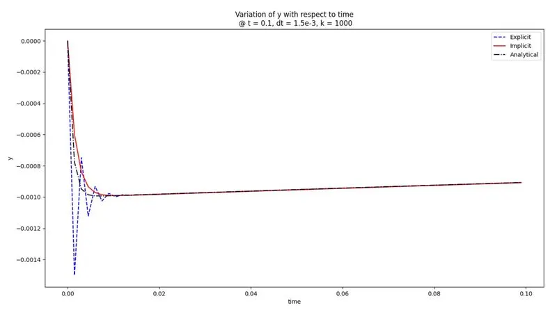
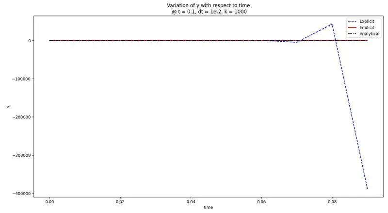
COMPARING AT SAME TIME STEP WITH DIFFERENT INPUTS:

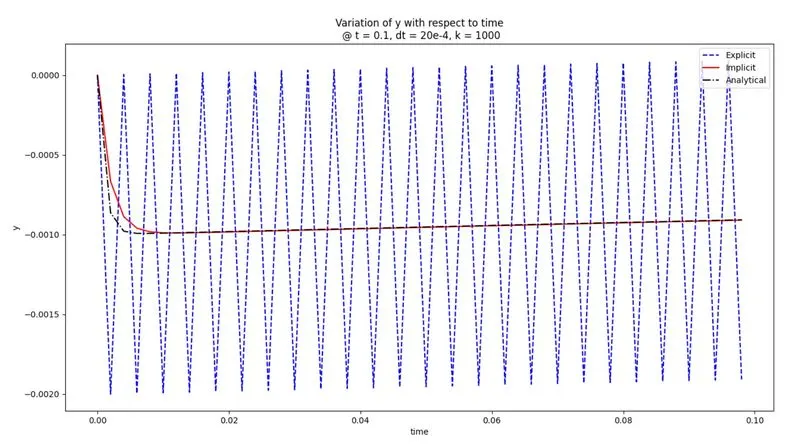
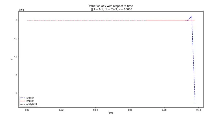
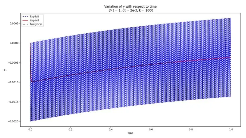
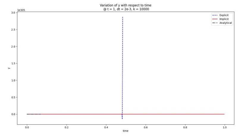
When does a ODE become unstable?

From the above plots, we can get to know that the solution is getting unstable only for explicit schemes. In initial situations, the solution is matching with the analytical solution when the time step is very large value for the give time but when the value of time step becoming small, the solution is blowing out for explicit scheme. Where as for implicit schemes, the solution is matching with the analytical solution even though the time step is small.

Thus,we can understand that the numerical stability has to do with the behavior of the solution as the time-step dt is increased. If the solution remains well behaved for arbitrarily large values of the time step, the method is said to be unconditionally stable. This situation never occurs with explicit methods, which are always conditionally stable. For explicit schemes,there must be some limit on the size of the time step for there to be a solution.

How does stability affect engineering simulations?

The unstable solution gives us a error which grows exponentially if we run the simulation for long time, this can be seen from the plot at which t = 1, dt = 2e-3. As the error becomes more which gives an unphysical solution which can't be usefull for real engineering simulations. When the solution is stable, the errrors raising for each iteration is going to reduce over some time steps until the solution reaches steady state which is usefull for engineering aspects.

Can stability condition be derived for all types of problems?

Stability condition can be derived for linear type of ODE systems only, if the problems is of PDE's then we can use the Either Eigen value analysis or else Von Neuman stability analysis. In Eigen value analysis, we create the jacobian matrix and compute the values fof the eigen values, if the eigen values are negative then the solution is stable or else unstable. When it comes to later analysis, it is used when the system domain is peroidic.In order for the differencing scheme to be stable, the modulus of this amplification factor must be less than unity for all possible values of wave length.