Week 5.2 - Literature review: ODE Stability

AIM:

Analysis of the stability of ODE solvers

THEORY:

Ordinary differential equation (ODE) is a differential equation containing one or more functions of one independent variable and the derivatives of those functions.

ODE can be solved using numerical methods. In solving engineering problems, the system of ODE can be coupled or uncoupled and cannot be solved directly. The numerical methods are implemented to solve those equations.

The numerical schemes can be classified into explicit and implicit schemes.

For explicit schemes, the value of a variable is calculated using the known values from the previous time steps.

For implicit schemes, the iterative techniques are used to solve the coupled set of equations.

When does ODE become stable?

The explicit schemes becomes unstable because of its dependence on the size of time step. When the time step values are higher than the ideal value, oscillations are observed.

The implicit schemes are highly stable because it uses iterative techniques for a given time step.

FOR EXAMPLE:

`dy/dt= -1000y-e^(-t)`

The equation is discretized as

`dy/dt= (y^n-y^(n-1))/(trianglet)`

Where, n is time step

`trianglet` is time step size

FOR EXPLICIT,

`(y^n-y^(n-1))/(triangle t)= -1000y^(n-1)-e^(-t^n )`

`y^n = (1-1000trianglet)y^(n-1) – e^-(t^n)trianglet`

FOR IMPLICIT,

`(y^n-y^(n-1))/(triangle t)= -1000y^(n-1)-e^(-t^n )`

`y^n= (y^(n-1)-e^(-t^n))/(1+1000triangle t)`

ANALYTICAL SOLUTION:

`y= (e^(-1000t)-e^(-t))/999`

CODING APPROACH:

• Importing the matplolib, cantera and numpy modules.
• The function explicit, implicit and analytical are defined.
• The numerical method or equation is defined for all the above functions.
• Then the time step is defined.
• Then the outputs are stored in t and y variable.
• Then the plot is made between time and Y for all the three functions.
• The legends, title and labels are defined for the plots.

CODE:

import matplotlib.pyplot as plt
import math
import numpy as np


def explicit(total_t,dt):
 	t = np.arange(0,total_t,dt)
 	y = np.zeros(len(t))

 	for i in range(1,len(t)):
 		y[i] = y[i-1] + dt*(-1000*y[i-1] - np.exp(-t[i-1]))
 	return [t,y]


def implicit(total_t,dt):
 	t = np.arange(0,total_t,dt)
 	y = np.zeros(len(t))

 	for i in range(1,len(t)):
 		y[i] = (y[i-1] - dt*np.exp(-t[i]))/(1+1000*dt)
 	return [t,y]


def analytical(total_t,dt):
 	t = np.arange(0,total_t,dt)
 	y = np.zeros(len(t))

 	for i in range(1,len(t)):
 		y[i] = (np.exp(-1000*t[i]) - np.exp(-t[i]))/999
 	return [t,y]

total_t = 0.1
dt = 0.0005
t,y_explicit = explicit(total_t,dt)
t,y_implicit = implicit(total_t,dt)
t,y_analytical = analytical(total_t,dt)
plt.plot(t,y_explicit,color='red')
plt.plot(t,y_implicit,color='blue')
plt.plot(t,y_analytical,color='green')
plt.xlabel('time(sec)')
plt.ylabel('y')
plt.title('timestep size :' + str(dt))
plt.legend(['explicit','implicit','analytical'])
plt.show()

RESULTS:

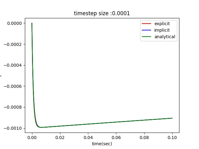
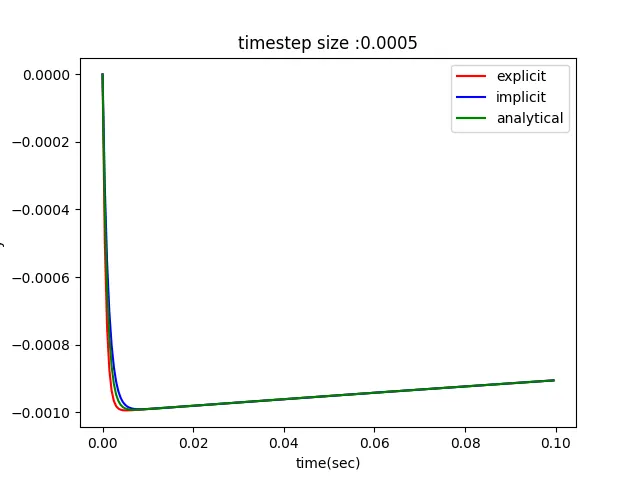
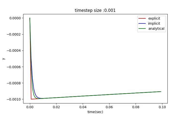
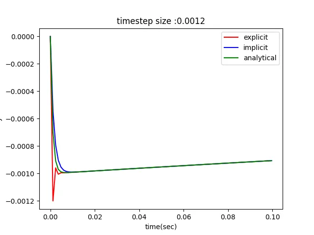
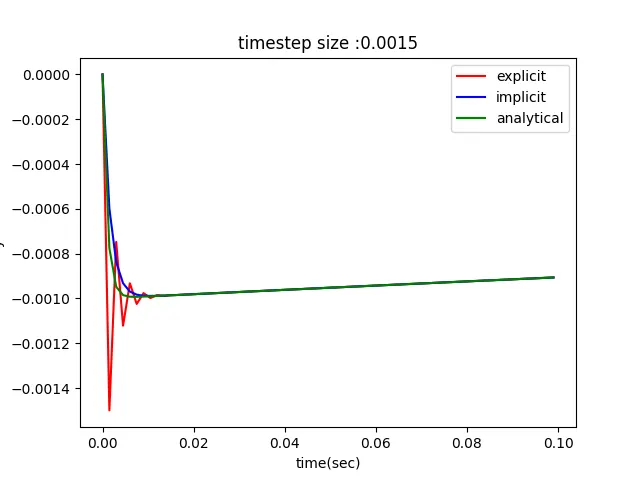
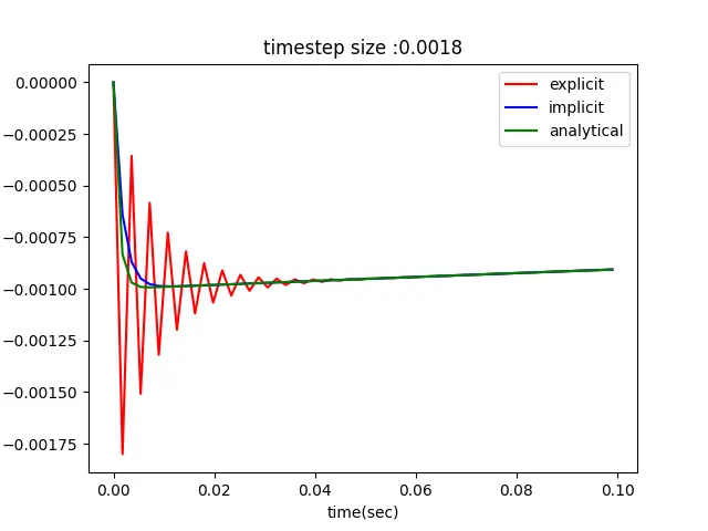
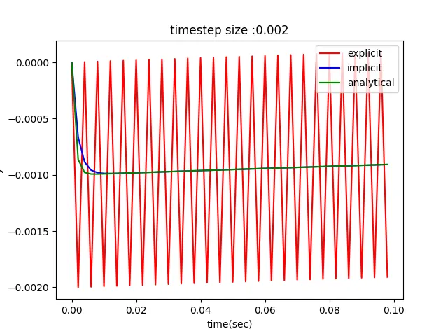
From the above plots we can see that explicit scheme starts to oscillate when time step start increasing from 1e-4 and the solution blows up. The timestep is the major factor which decides the solution is stable or not.The implicit schemes are unconditionally stable and doesnot depends on time step.

How does stability affect engineering simulations?

In engineering simulations, a stable method should be chosen to obtain the solution. If we doesn’t select the stable method the solution would be mathematically correct but not accurate. Hence a proper scheme needs to be adopted for obtaining accurate results.

Can stability conditions be derived for all type of problems?

Stability conditions can be derived for all type of problems.

There are two common stability conditions they are

• Eigen value stability condition
• Von-neuman stability condition