Week 5.2 - Literature review: ODE Stability

Aim: To write a literature review on the stability of ODE and to answer the following questions

• When does an ODE become unstable?
• How does stability affect engineering simulations?
• Can stability conditions be derived for all types of problems?

Introduction:

An equation containing one or more functions of one independent variable and its derivatives is called an ordinary differential equation.

The ordinary differential equations are majorly classified as:

• Autonomous ODE
• Linear ODE
• Non-linear ODE

Solving the ordinary differential equation can be done explicitly or implicitly.

When does an ODE become unstable:

Unstable ode is defined as the ode with the solution diverging i.e the perturbations increasing or diverging. the ODE becomes unstable when the step size is large and sometimes larger than the difference between the solution of the consecutive iterations.

The Implicit schemes are independent of the time step size and are unconditionally stable. There will be no stability in the explicit schemes irrespective of the time step. Time step plays an important role in the numerical methods, especially in the explicit schemes. The odes become unstable with the increasing time step.

How does stability affect engineering simulations?

The stability of the ODE's is important in engineering simulations. The ode's stability helps engineers concentrate on the solution and make modifications in the inputs to get a required solution. Stability in the ode helps in comparing the results of the numerical solution with the analytical solution. The stability of the ode also depends on the boundary conditions and the initial values.

Though the implicit schemes are unconditionally stable they take longer time and simulation capacity so the boundary conditions and time steps should be chosen wisely. The divergence of the solution greatly depends on the boundary conditions if the boundary conditions are not given the solution may never converge.

Unstable Odes give unstable solutions that are unphysical results that cant be trusted

Can stability conditions be derived for all types of problems?

Implicit schemes are unconditionally stable so we can derive stability conditions for most problem types. Though the Implicit schemes are superior to the explicit schemes inaccuracy they tend to consume more computational power and time to give the results, so sometimes explicit schemes are preferred where the accuracy is not the priority to get the solution quickly.

To show it in the plots an ode is used and solved using eulers method.

ODE

`dy/dt=-1000y-exp(-t) when y(0)=0`

Explicit solution

`y^(n+1)=(-1000y^(n)-e^(-t))*dt+y(n)`

Explicit solution

`y^(n+1)=(y^(n)-e^(-t)*dt)/(1+1000*dt)`

Analytical solution

`y(t) = (e^(-1000 t) (1 - e^(999 t)))/999`

Code:

#Literature review On ODE
import math
import matplotlib.pyplot as plt
import numpy as np
# Numerical solving
def explicit_euler(t_total,dt):
	t=np.arange(0,t_total,dt)
	y=np.zeros(len(t))
	

	for i in range(1,len(t)):
		y[i]=y[i-1]+dt*(-1000*y[i-1]-np.exp(-t[i-1]))
	return [t,y]

def implicit_euler(t_total,dt):
	t=np.arange(0,t_total,dt)
	y=np.zeros(len(t))

	for i in range(1,len(t)):
		y[i]=(y[i-1]-np.exp(-t[i-1])*dt)/(1+1000*dt)

	return [t,y]
# analytical Solving
def analytical_euler(t_total,dt):
	t=np.arange(0,t_total,dt)
	y=np.zeros(len(t))

	for i in range(1,len(t)):
		y[i]=np.exp(-1000*t[i])*(1 - np.exp(999*t[i]))/999

	return [t,y]
# Total time 
t_total=0.1
dt=5e-3
t,y_explicit=explicit_euler(t_total,dt)
t,y_implicit=implicit_euler(t_total,dt)
t,y_analytical=analytical_euler(t_total,dt)
plt.plot(t,y_explicit,'--',color='blue')
plt.plot(t,y_implicit,'--.',color='yellow')
plt.plot(t,y_analytical,'-.',color='red')
plt.xlabel('T')
plt.ylabel('y')
plt.legend(['Explicit Method','Implicit Method','analytical Method'])
plt.show()

Plots:

plots are results of varying time step sizes of Explicit, Implicit, and analytical solutions.

Step size is 1e^-4

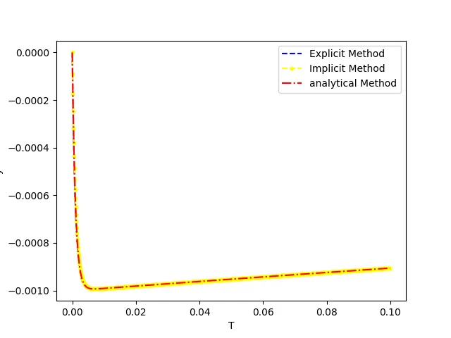
Both the explicit and implicit methods solutions are close to Analytical solution and solutions are stable and accurate.

Step size is 1.2e^-3

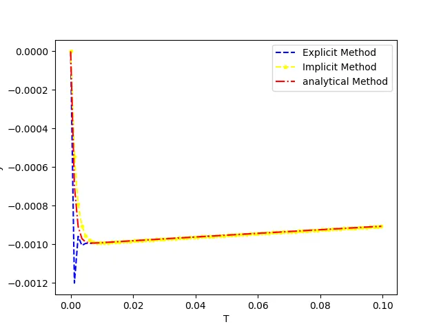
the explicit solution becomes stable after some time.

Step size is 1.9e^-3

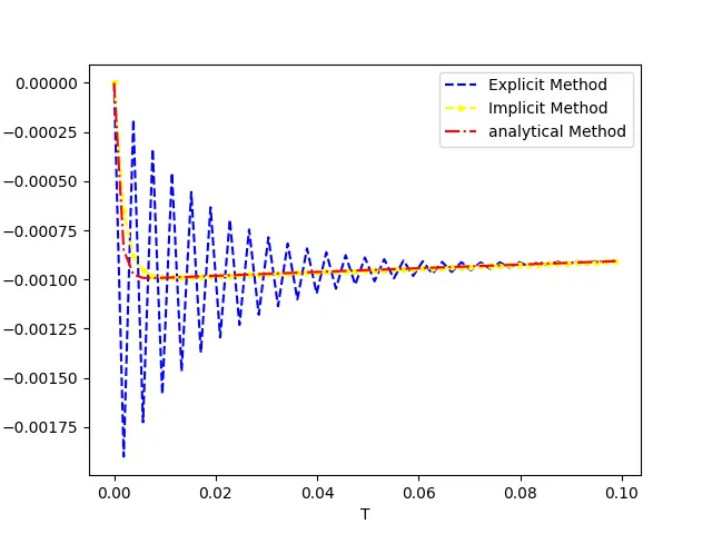
The explicit solution is unstable at attains stability after some time.

Step size is 5e^-3

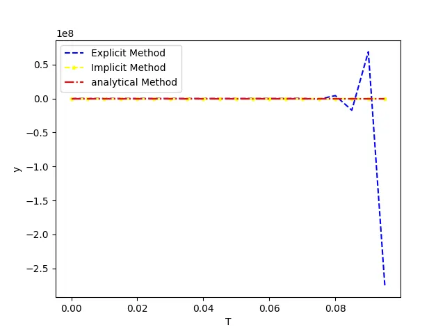
the explicit solution has diverged and it is impossible to get stable. The implicit solution is stable.

if dt is greater than total time /constant the explicit solution becomes unstable,The constant is 1000

if dt is less than total time /constant the explicit solution becomes stable

Conclusion:
The explicit solutions are stable until the time step is lower than the certain Critical value and if the time step is large the solution gets diverged. For larger time steps the Implicit method gives stable results but might not be accurate.