Rankine cycle Simulator

Aim:

To create a Rankine cycle simulator using Matlab/Octave.

Rankine cycle or Steam Turbine cycle:

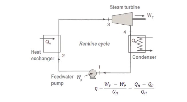
the Rankine cycle is an idealized thermodynamic cycle of a constant pressure heat engine that converts part of heat into mechanical work. In this cycle, the heat is supplied externally to a closed loop, which usually uses water (in a liquid and vapor phase) as the working fluid.

Rankine Cycle – Processes

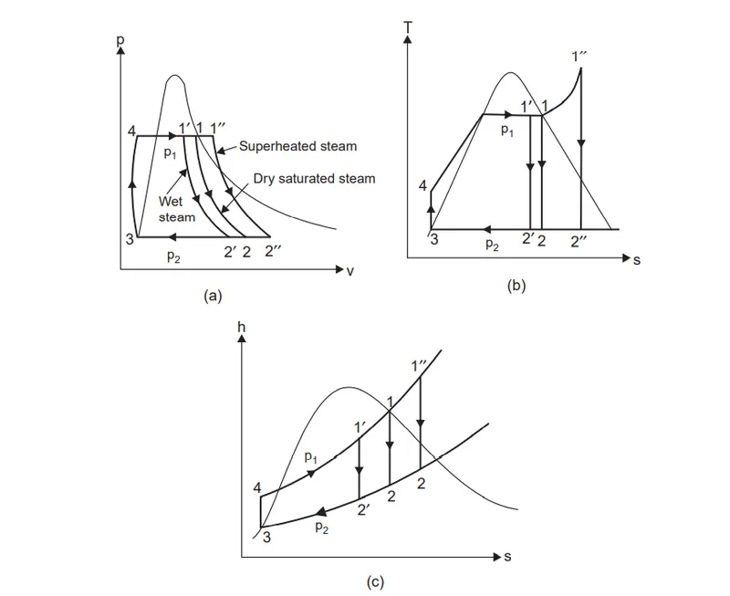
• Isentropic compression (compression in centrifugal pumps) – The liquid condensate is compressed adiabatically from state 1 to state 2 by centrifugal pumps (usually by condensate pumps and then by feedwater pumps). The liquid condensates s pumped from the condenser into the higher pressure boiler. In this process, the surroundings do work on the fluid, increasing its enthalpy (h = u+pv) and compressing it (increasing its pressure). On the other hand, the entropy remains unchanged. The work required for the compressor is given by W_Pumps = H₂ – H₁.
• Isobaric heat addition (in a heat exchanger – boiler) – In this phase (between state 2 and state 3), a constant-pressure heat transfer to the liquid condensate from an external source, since the chamber is open to flow in and out. The feedwater (secondary circuit) is heated to the boiling point (2 → 3a) of that fluid and then evaporated in the boiler (3a → 3). The net heat added is given by Q_add = H₃ – H₂
• Isentropic expansion (expansion in a steam turbine) – Steam from the boiler expands adiabatically from state 3 to state 4 in a steam turbine to produce work and then is discharged to the condenser (partially condensed). The steam does work on the surroundings (blades of the turbine) and loses an amount of enthalpy equal to the work that leaves the system. The work done by a turbine is given by W_T = H₄ – H₃. Again the entropy remains unchanged.
• Isobaric heat rejection (in a heat exchanger) – In this phase, the cycle completes by a constant-pressure process in which heat is rejected from the partially condensed steam. There is heat transfer from the vapor to cooling water flowing in a cooling circuit. The vapor condenses and the temperature of the cooling water increases. The net heat rejected is given by Qre = H₄ – H₁

During a Rankine cycle, work is done on the fluid by the pumps between states 1 and 2 (isentropic compression). Work is done by the fluid in the turbine between stages 3 and 4 (isentropic expansion). The difference between the work done by the fluid and the work done on the fluid is the net work produced by the cycle and it corresponds to the area enclosed by the cycle curve (in PV diagram). The working fluid in a Rankine cycle follows a closed loop and is reused constantly.

Isobaric process (Vdp = 0):

dH = dQ → Q = H₂ – H₁

At constant entropy, i.e. in the isentropic process, the enthalpy change equals the flow process work done on or by the system:

Isentropic process (dQ = 0):

dH = Vdp → W = H₂ – H₁

_{Isentropic process:}

An isentropic process is a thermodynamic process, in which the entropy of the fluid or gas remains constant. It means the isentropic process is a special case of an adiabatic process in which there is no transfer of heat or matter. It is a reversible adiabatic process. The assumption of no heat transfer is very important since we can use the adiabatic approximation only in very rapid processes.

Isentropic Process and the First Law

For a closed system, we can write the first law of thermodynamics in terms of enthaply

dH = dQ + Vdp

or

dH = TdS + Vdp

Isentropic process (dQ = 0):

dH = Vdp → W = H₂ – H₁

Isobaric Process

An isobaric process is a thermodynamic process, in which the pressure of the system remains constant (p = const). The heat transfer into or out of the system does work and changes the system's internal energy.

Since there are changes in internal energy (dU) and changes in system volume (∆V), engineers often use the enthalpy of the system, which is defined as:

H = U + pV

Isobaric Process and the First Law

The classical form of the first law of thermodynamics

dU = dQ – dW

In this equation, dW is equal to dW = pdV and is known as the boundary work. In an isobaric process and the ideal gas, part of the heat added to the system will be used to do work and part of the heat added will increase the internal energy (increase the temperature). Therefore it is convenient to use enthalpy instead of internal energy.

Isobaric process (Vdp = 0):

dH = dQ → Q = H₂– H₁

At constant entropy, i.e. in isentropic process, the enthalpy change equals the flow process work done on or by the system.

Program:

clear all
close all
clc

% Displaying 
fprintf('%50sn','RANKINE CYCLE SIMULATOR')
fprintf('n')
fprintf('%sn','Process 1-2 Reversible adiabatic expansion in the turbine.')
fprintf('%sn','Process 2-3 Constant pressure transfer of heat in the condenser.')
fprintf('%sn','Process 3-4 Reversible adiabatic pumping process in the feed pump.')
fprintf('%sn','Process 4-1 Constant pressure transfer of heat in the boiler.')

fprintf('n')
%Input

% t1=400;
% p1=30;
% p2=0.05;

p1=input('Enter the Pressure at the Turbine inlet (in bar):');

t1=input('Enter the Temperature at the Turbine inlet( Degree celcius):');

p2=input('Enter the Pressure at the Condenser (bar):');



%Calculating state variables at point 1:
h1=XSteam('h_pT',p1,t1);
s1=XSteam('s_pT',p1,t1);

%Calculating state variables at point 2:
s2=s1; %reversible adiabatic expansion
%s2=sf2+x2.sfg2
%sfg2=sg2-sf2
sf2=XSteam('sL_p',p2);
sg2=XSteam('sV_p',p2);
x2=(s2-sf2)/(sg2-sf2);
%h2=hf2+x2(hfg2)
%h2=hf2+x2(hg2-hf2)
hg2=XSteam('hV_p',p2);
hf2=XSteam('hL_p',p2);
h2=hf2+x2*(hg2-hf2);

% Turbine_work 
wt=h1-h2;

%Calculating state varaible at point 3:
p3=p2; %Constant pressure transfer of heat in the condenser
h3=XSteam('hL_p',p3);
s3=XSteam('sL_p',p3);
t3=XSteam('Tsat_p',p3);
t2=t3;

%Calculating state variable at point 4:
s4=s3; % Constant entropy
p4=p1; % Constant pressure

% Pump_work
%wp=hf4-hf3;
%wp=v3(p1-p2);
v3=XSteam('vL_p',p3);
wp=v3*(p1-p2)*100;
h4=XSteam('h_ps',p4,s4);
t4=XSteam('T_ps',p4,s4);

%calculating state variable at point 5
p5=p4;
t5=XSteam('Tsat_p',p5);
h5=XSteam('hL_p',p5);
s5=XSteam('sL_p',p5);

% Calculating state variable at point 6
t6=t5;
p6=XSteam('psat_T',t6);
h6=XSteam('hV_T',t6);
s6=XSteam('sV_T',t6);


%Net work
w_net=wt-wp;
%heat input
q_in=h1-h4;
%heat output
q_out=h2-h3;
%thermal_eff
Ntherm=w_net/q_in;

%Work ratio
work_ratio=w_net/wt;    


%Saturation curve

t=linspace(1,375,1000);
for i=1:length(t)
    sf(i)=XSteam('sL_T',t(i));
    sg(i)=XSteam('sV_T',t(i));
    hf(i)=XSteam('hL_T',t(i));
    hg(i)=XSteam('hV_T',t(i));
end

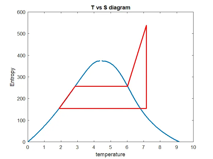
%Plotting t-s
figure(1)
plot([sf,sg],[t,t],'linewidth',2)
hold on
plot([s1,s2,s3,s4,s5,s6],[t1,t2,t3,t4,t5,t6],'linewidth',2,'color','r')
plot([s1,s6],[t1,t6],'linewidth',2,'color','r')
xlabel('temperature')
ylabel('Entropy')
title('T vs S diagram')

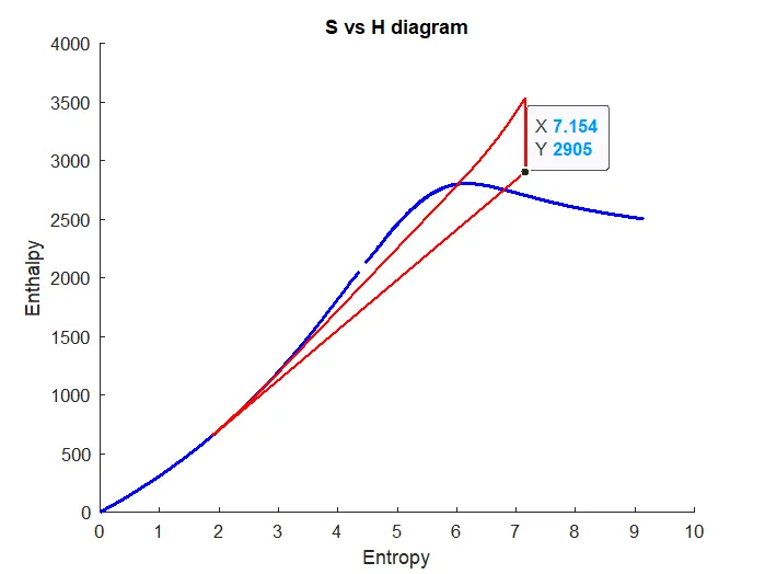
%plotting s h
figure(2)
hold on 
plot(sg,hg,'linewidth',2,'color','b')
plot(sf,hf,'color','b','linewidth',2,'color','b')
plot([s1,s2,s3,s4],[h1,h2,h3,h4],'linewidth',1,'color','r')

hc=linspace(h4,h5,100);
for r=1:length(hc)
    sch(r)=XSteam('s_ph',p1,hc(r));
end
plot(sch,hc,'linewidth',1,'color','r')
plot([s5,s6],[h5,h6],'r','linewidth',1,'color','r')
sc1=linspace(s6,s1,1000);
for m=1:length(sc1)
    hc1(m)=XSteam('h_ps',p1,sc1(m));
end
plot(sc1,hc1,'linewidth',1,'color','r')
xlabel('Entropy')
ylabel('Enthalpy')
title('S vs H diagram')

%Displaying result
fprintf('%10sn','Results')
fprintf('At State Point 1:n')
fprintf('p1 is :%3.2f barn',p1)
fprintf('t1 is :%3.2f Deg Celciusn',t1)
fprintf('s1 is :%3.2f kJ/KgKn',s1)
fprintf('h1 is :%3.2f kJ/kgn',h1)

fprintf('n')
fprintf('At State Point 2:n')
fprintf('p2 is :%3.2f barn',p2)
fprintf('t2 is :%3.2f Deg Celciusn',t2)
fprintf('s2 is :%3.2f kJ/KgKn',s2)
fprintf('h2 is :%3.2f kJ/kgn',h2)

fprintf('n')
fprintf('At State Point 3:n')
fprintf('p3 is :%3.2f barn',p3)
fprintf('t3 is :%3.2f Deg Celciusn',t3)
fprintf('s3 is :%3.2f kJ/KgKn',s3)
fprintf('h3 is :%3.2f kJ/kgn',h3)

fprintf('n')
fprintf('At State Point 4:n')
fprintf('p4 is :%3.2f barn',p4)
fprintf('t4 is :%3.2f Deg Celciusn',t4)
fprintf('s4 is :%3.2f kJ/KgKn',s4)
fprintf('h4 is :%3.2f kJ/kgn',h4)

fprintf('n')
fprintf('wt is:%3.2f kJ/kgn',wt)
fprintf('wp is:%3.2f kJ/kgn',wp)
fprintf('w_net is:%f3 kJ/kgn',w_net)
fprintf('Ntherm is:%f3 percentn',Ntherm)

plots:

Result:

                           RANKINE CYCLE SIMULATOR

Process 1-2 Reversible adiabatic expansion in the turbine.
Process 2-3 Constant pressure transfer of heat in the condenser.
Process 3-4 Reversible adiabatic pumping process in the feed pump.
Process 4-1 Constant pressure transfer of heat in the boiler.

Enter the Pressure at the Turbine inlet (in bar):44
Enter the Temperature at the Turbine inlet( Degree celcius):538
Enter the Pressure at the Condenser (bar):5.38
   Results
At State Point 1:
p1 is :44.00 bar
t1 is :538.00 Deg Celcius
s1 is :7.15 kJ/KgK
h1 is :3528.83 kJ/kg

At State Point 2:
p2 is :5.38 bar
t2 is :154.62 Deg Celcius
s2 is :7.15 kJ/KgK
h2 is :2904.52 kJ/kg

At State Point 3:
p3 is :5.38 bar
t3 is :154.62 Deg Celcius
s3 is :1.89 kJ/KgK
h3 is :652.21 kJ/kg

At State Point 4:
p4 is :44.00 bar
t4 is :155.06 Deg Celcius
s4 is :1.89 kJ/KgK
h4 is :656.45 kJ/kg

wt is:624.31 kJ/kg
wp is:4.23 kJ/kg
w_net is:620.0777863 kJ/kg
Ntherm is:0.2158763 percent

Error:

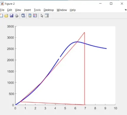this is due to the wrong formula was stated for s1 and h1.

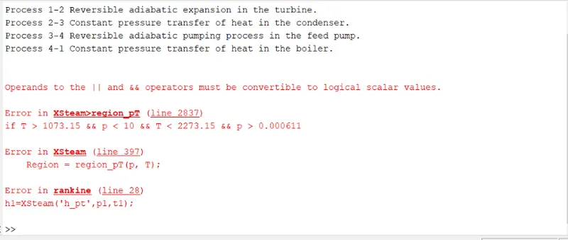
Typo in while stating inputs

Reference:

https://www.thermal-engineering.org/what-is-rankine-cycle-steam-turbine-cycle-definition/