Week 5.1 - Mid term project - Solving the steady and unsteady 2D heat conduction problem

Objective:

To perform a Steady-state analysis & Transient State Analysis to solve the 2D heat conduction equation by using the point iterative techniques.

Steady State:

Main code:

clear all
close all
clc
%Initialising boundary condition
    T_top = 600;
    T_left = 400;
    T_right = 800;
    T_bottom = 900;
%Initialising Guess value    
    T_guess = 300;
%Discretising the domain    
    no_div = 10;
    nodes = linspace(0,1,no_div);
    dx = nodes(2)-nodes(1);
    dy = dx;
%computing constant
    k = (dy^2*dx^2)/(2*(dx^2+dy^2));

%Initializing the domain with guessed value
    domain = T_guess*ones(length(nodes));
    
%create a rectangular grid out of two given one-dimensional arrays    
    [xx,yy] = meshgrid(nodes,nodes);
%Applying boundary condition to all nodes
    domain(1,2:(length(nodes)-1)) = T_top;
    domain(2:(length(nodes)-1),1) = T_left;
    domain(length(nodes),2:(length(nodes)-1)) = T_bottom;
    domain(2:(length(nodes)-1),length(nodes)) = T_right;

    domain(1,1) = (T_top+T_left)/2;
    domain(length(nodes),length(nodes)) = (T_bottom+T_right)/2;
    domain(1,length(nodes)) = (T_top+T_right)/2;
    domain(length(nodes),1) = (T_bottom+T_left)/2;
%Alloting the values of domain to T variable for computation    
    T = domain;
%%
%%
c_1 = clock ;   
[T_jacobi,Iter_jacobi] = steady_jacobi(nodes,T,k,dx);
c_2 = clock ;
time = c_2-c_1;
elapsed_time_jacobi = sum(3600*time(4)+60*time(5)+time(6));
figure(1)
C_1 = contourf(xx,yy,T_jacobi);
clabel(C_1,'FontWeight','bold'); 
set(gca,'YDIR','reverse')
title_text=sprintf('Jacobi');
title(title_text)
%%
%%
c_1 = clock ;
[T_gs,Iter_gs] = steady_gs(nodes,T,k,dx);
c_2 = clock ;
time = c_2-c_1;
elapsed_time_gs = sum(3600*time(4)+60*time(5)+time(6));
figure(2)
C_2 = contourf(xx,yy,T_gs);
clabel(C_2,'FontWeight','bold'); 
set(gca,'YDIR','reverse')
title_text=sprintf('Gauss Seidel');
title(title_text)
%%
%%
c_1 = clock ;
[T_sor,Iter_sor] = steady_sor(nodes,T,k,dx);
c_2 = clock ;
time = c_2-c_1;
elapsed_time_sor = sum(3600*time(4)+60*time(5)+time(6));
figure(3)
C_3 = contourf(xx,yy,T_sor);
clabel(C_3,'FontWeight','bold'); 
set(gca,'YDIR','reverse')
title_text=sprintf('Successive Over Relaxation');
title(title_text)

%%

X = categorical({'Jacobi','Gauss Seidel','SOR'});
X = reordercats(X,{'Jacobi','Gauss Seidel','SOR'});
figure(4)
Iter_count = [Iter_jacobi Iter_gs Iter_sor];
bar(X,Iter_count)
title('Iteration Count')

figure(5)
Iter_time = [elapsed_time_jacobi elapsed_time_gs elapsed_time_sor];
bar(X,Iter_time)

Function Code(Implicit):

• Jacobi

function [T_out,e_jac] = steady_jacobi(nodes,T,k,dx)
%Discretising the domain
    dy = dx;
%Alloting the values of domain to T variable for computation    
    T_old = T;
%Initialising the iteration count    
    e_jac = 0;
%Initialising the tolerance and error values
    tolerance = 1.0000e-04;
    error = 1;   
%while loop to check for convergance    
    while (error>tolerance)
%Space loop
        for i = 2:(length(nodes)-1)
            for j = 2:(length(nodes)-1)
            term_1 = (T_old(i,j-1)+T_old(i,j+1))/dx^2;
            term_2 = (T_old(i-1,j)+T_old(i+1,j))/dy^2;
                T(i,j) = (term_1+term_2)*k;
            end
        end
%Computing of error       
    error = max(max(abs(T_old-T)));
    T_old = T;
    e_jac = e_jac+1
    end
%Output of the function    
    T_out = T;
end

• Gauss-Seidel:

function [T_out,e_gs] = steady_gs(nodes,T,k,dx)
%Discretising the domain
    dy = dx;
%Alloting the values of domain to T variable for computation    
    T_old = T;
%Initialising the iteration count    
    e_gs = 0;
%Initialising the tolerance and error values
    tolerance = 1.0000e-04;
    error = 1;   
%while loop to check for convergance    
    while (error>tolerance)
%Space loop
            for i = 2:(length(nodes)-1)
                for j = 2:(length(nodes)-1)
                    term_1 = (T(i,j-1)+T_old(i,j+1))/dx^2;
                    term_2 = (T(i-1,j)+T_old(i+1,j))/dy^2;
                    T(i,j) = (term_1+term_2)*k;
                end
            end
%Computing of error                 
error = max(max(abs(T_old-T)));
T_old = T;
e_gs = e_gs+1
    end
%Output of the function    
    T_out = T;
end

• SOR:

function [T_out,e_sor] = steady_sor(nodes,T,k,dx)
%Relaxation fctor    
    w = 1.8;
%Discretising the domain
    dy = dx;
%Alloting the values of domain to T variable for computation    
    T_old = T;
%Initialising the iteration count    
    e_sor = 0;
%Initialising the tolerance and error values
    tolerance = 1.0000e-04;
    error = 1;   
%while loop to check for convergance    
    while (error>tolerance)
%Space loop
        for i = 2:(length(nodes)-1)
            for j = 2:(length(nodes)-1)
                term_1 = (T(i,j-1)+T_old(i,j+1))/dx^2;
                term_2 = (T(i-1,j)+T_old(i+1,j))/dy^2;
                T(i,j) = (1-w)*T_old(i,j)+w*(term_1+term_2)*k;
            end
        end
%Computing of error          
    error = max(max(abs(T_old-T)));
    T_old = T;
    e_sor = e_sor+1
    end
%Output of the function    
    T_out = T;
end
    

Transient State:

Main code:

clear all
close all
clc

T_top = 600;
T_left = 400;
T_right = 800;
T_bottom = 900;
T_guess = 300;
no_div =10;

nodes = linspace(0,1,no_div);
dx = nodes(2)-nodes(1);

domain = T_guess*ones(length(nodes));
[xx,yy] = meshgrid(nodes,nodes);

domain(1,2:(length(nodes)-1)) = T_top;
domain(2:(length(nodes)-1),1) = T_left;
domain(length(nodes),2:(length(nodes)-1)) = T_bottom;
domain(2:(length(nodes)-1),length(nodes)) = T_right;

domain(1,1) = (T_top+T_left)/2;
domain(length(nodes),length(nodes)) = (T_bottom+T_right)/2;
domain(1,length(nodes)) = (T_top+T_right)/2;
domain(length(nodes),1) = (T_bottom+T_left)/2;

% 
% display =('Enter any one of the options and press Enter')
% % method 1 = jacobi solver, 2 = Gauss Seidel Solver & 3 = SOR method.
% prompt= 'Choose iterative solver type 1 = Explicit 2 = Implicit jacobi solver, 3 = Implicit Gauss Seidel Solver & 4 = Implicit SOR method\n';
% method = input(prompt); 

%%
c_1 = clock ;     
[T_out_explicit] = Unsteady_explicit(dx,domain);
c_2 = clock ;
time = c_2-c_1;
elapsed_time_explicit = sum(3600*time(4)+60*time(5)+time(6));
figure(1)
C=contourf(xx,yy,T_out_explicit);
clabel(C,'FontWeight','bold'); 
set(gca,'YDIR','reverse')
title_text=sprintf('Unsteady explicit');
title(title_text)

%%
%%
c_1 = clock ;    
[T_out_implicit_jacobi,iter_jacobi] = Unsteady_implicit_jacobi(dx,domain);
c_2 = clock ;
time = c_2-c_1;
elapsed_time_jacobi = sum(3600*time(4)+60*time(5)+time(6));
figure(2)
C_1=contourf(xx,yy,T_out_implicit_jacobi);
clabel(C_1,'FontWeight','bold'); 
set(gca,'YDIR','reverse')
title_text=sprintf('Jacobi');
title(title_text)
%%
%%
c_1 = clock ;    
[T_out_implicit_gausssiedel,iter_gs] = Unsteady_implicit_gausssiedel(dx,domain);
c_2 = clock ;
time = c_2-c_1;
elapsed_time_gausssiedel = sum(3600*time(4)+60*time(5)+time(6));
figure(3)
C_2=contourf(xx,yy,T_out_implicit_gausssiedel);
clabel(C_2,'FontWeight','bold'); 
set(gca,'YDIR','reverse')
title_text=sprintf('Gauss Seidel');
title(title_text)
%%
%%
c_1 = clock ;     
[T_out_implicit_sor,iter_sor] = Unsteady_implicit_sor(dx,domain);
c_2 = clock ;
time = c_2-c_1;
elapsed_time_sor= sum(3600*time(4)+60*time(5)+time(6));
figure(4)
C_3=contourf(xx,yy,T_out_implicit_sor);
clabel(C_3,'FontWeight','bold'); 
set(gca,'YDIR','reverse')
title_text=sprintf('Successive Over Relaxation');
title(title_text)
%%

X = categorical({'Jacobi','Gauss Seidel','SOR'});
X = reordercats(X,{'Jacobi','Gauss Seidel','SOR'});
figure(4)
Iter_count = [iter_jacobi iter_gs iter_sor];
bar(X,Iter_count)
title('Iteration Count')

figure(5)
X = categorical({'explicit','Jacobi','Gauss Seidel','SOR'});
X = reordercats(X,{'explicit','Jacobi','Gauss Seidel','SOR'});
Iter_time = [elapsed_time_explicit elapsed_time_jacobi elapsed_time_gausssiedel elapsed_time_sor];
bar(X,Iter_time)

Function Code:

• Explicit:

function [T_out] = Unsteady_explicit(dx,domain)

%Defining the old and new temperature profile
    T_old = domain;
    T = domain;
    
%Since square domain the dy = dx    
    dy = dx;
    
%Defining value of Thermal diffusivity
    alpha = 1.5;
    
%time step size such that the sum total of k_1 and k_2 is less than 0.5
    dt = 0.22*dx^2/alpha;
    
%flow time
    t = 1.4;
    
%no.of time step
    nt = t/dt;

%Defining the vlue of constants
    k_1 = alpha*dt/dx^2;
    k_2 = alpha*dt/dy^2;

%Time loop    
    for time = 1:nt
%Space loop
        for i = 2:length(domain)-1
            for j = 2:length(domain)-1
                T(i,j) = T_old(i,j)*(1-2*k_1-2*k_2)+k_1*(T_old(i,j+1)+T_old(i,j-1))+k_2*(T_old(i+1,j)+T_old(i-1,j));
                        
            end
        end
%Replacing new value of temperature as teperature at old timestep
    T_old = T;
 
    end
%Defining the final profile of temperature as output
    T_out = T;

end

            

• Jacobi(implicit):

function [T_out,e_jacobi] = Unsteady_implicit_jacobi(dx,domain)
%%%%%%%%%%%%%%%%%%%%%%%%%%%%%%%%%%%%%%%%%%%%%%%%%%%%%%%%%%%%%%%%%%%%%%%%%%%%%%%%%%%%%%%%
e_jacobi = 0;
%Since square domain the dy = dx   
    dy = dx;
    
%Defining value of Thermal diffusivity
    alpha = 1.5;
    
%time step size
    dt = 0.36*dx^2/alpha;
    
%flow time
    t = 1.4;
    
%no.of time step
    nt = t/dt;
%Defining the value of constants     
    k_1 = alpha*dt/dx^2;
    k_2 = alpha*dt/dy^2;
    constant = 1/(1+2*k_1+2*k_2);
%Initializing the intial conditions of the temperature profile
    T_old = domain;
    T_new = domain;
    T = domain;

%Time loop 
    for u = 1:nt
%Initializing error and tolerance for each time step    
        error = 1000;
        tolerance= 1e-4;
%Checking for error with tolerance
            while error>tolerance
%Space loop
                for i = 2:length(domain)-1
                    for j = 2:length(domain)-1
                          T(i,j) = constant*(T_old(i,j)+k_1*(T_old(i,j-1)+T_old(i,j+1))+k_2*(T_old(i-1,j)+T_old(i+1,j)));           
                    end
                end
%Computing the error                   
    error = max(max(abs(T-T_old)));
%Replacing new value of temperature as teperature at old timestep        
    T_old = T;
   e_jacobi = e_jacobi+1 
            end
    end
%Defining the final profile of temperature as output
    T_out = T;

end

• Gauss-Seidel(implicit):

function [T_out,e_gausssiedel] = Unsteady_implicit_gausssiedel(dx,domain)
%%%%%%%%%%%%%%%%%%%%%%%%%%%%%%%%%%%%%%%%%%%%%%%%%%%%%%%%%%%%%%%%%%%%%%%%%%%%%%%%%%%%%%%%
e_gausssiedel = 0;
%Since square domain the dy = dx   
    dy = dx;
    
%Defining value of Thermal diffusivity
    alpha = 1.5;
    
%time step size
    dt = 0.36*dx^2/alpha;
    
%flow time
    t = 1.4;
    
%no.of time step
    nt = t/dt;
%Initializing the intial conditions of the temperature profile    
    T_old = domain;
    T_new = domain;
%Defining the value of constants
    k_1 = alpha*dt/dx^2;
    k_2 = alpha*dt/dy^2;
    constant = 1/(1+2*k_1+2*k_2);

%Time loop 
    for u = 1:nt
%Initializing error and tolerance for each time step    
    error = 1000;
    tolerance= 1e-4;
%Checking for error with tolerance
        while error>tolerance
%Space loop
            for i = 2:length(domain)-1
                for j = 2:length(domain)-1
                      T_new(i,j) = constant*(T_old(i,j)+k_1*(T_new(i,j-1)+T_old(i,j+1))+k_2*(T_new(i-1,j)+T_old(i+1,j)));           
                end
            end
%Computing the error    
    error = max(max(abs(T_new-T_old)));
%Replacing new value of temperature as teperature at old timestep        
    T_old = T_new;
    e_gausssiedel = e_gausssiedel+1
        end

    end
%Defining the final profile of temperature as output
    T_out = T_new;

end

            

• SOR(implicit):

function [T_out,e_sor] = Unsteady_implicit_sor(dx,domain)
%input the relaxation factor
    w = 1.8;

%%%%%%%%%%%%%%%%%%%%%%%%%%%%%%%%%%%%%%%%%%%%%%%%%%%%%%%%%%%%%%%%%%%%%%%%%%%%%%%%%%%%%%%%
e_sor = 0;
%Since square domain the dy = dx    
    dy = dx;
    
%time step size
    dt = 3e-3;
    
%flow time
    t = 1.4;
    
%no.of time step
    nt = t/dt;
    
%Defining value of Thermal diffusivity
    alpha = 1.5;
    
%Defining the value of constants    
    k_1 = alpha*dt/dx^2;
    k_2 = alpha*dt/dy^2;
    constant = 1/(1+2*k_1+2*k_2);

%Initializing the intial conditions of the temperature profile
    T_old = domain;
    T_new = domain;
    T_sor = domain;

%Time loop 
    for u = 1:nt
%Initializing rror and tolerance for each time step    
    error = 1000;
    tolerance= 1e-4;
%Checking for error with tolerance
        while error>tolerance
%Space loop            
            for i = 2:length(domain)-1
                for j = 2:length(domain)-1
                   T_new(i,j) = constant*(T_old(i,j)+k_1*(T_new(i,j-1)+T_old(i,j+1))+k_2*(T_new(i-1,j)+T_old(i+1,j)));          
                  T_sor(i,j) = (1-w)*T_old(i,j)+w*T_new(i,j);
                end
            end
%Computing the error            
    error = max(max(abs(T_sor-T_old)));
%Replacing new value of temperature as teperature at old timestep    
    T_old = T_sor;
%SOR iteration count    
    e_sor = e_sor+1
        end
    end
%Defining the final profile of temperature as output
    T_out = T_new;
end

            

Results:

Steady State:

• Jacobi:

• Gauss-Siedel:

• SOR:

Iteration count:

Transient State:

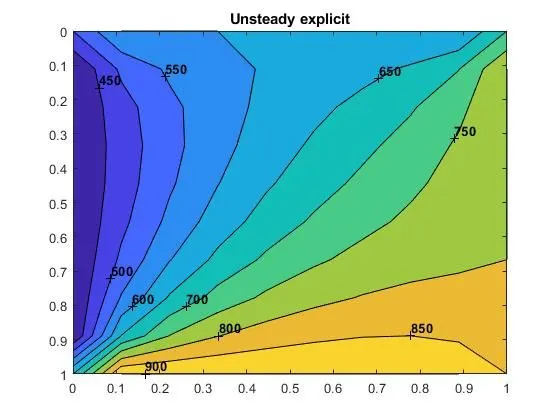
• Explicit

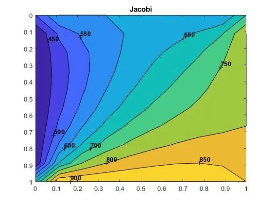
• Jacobi(Implicit):

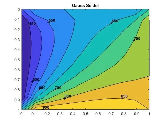
• Gauss-Siedel(Implicit):

• SOR(Implicit):

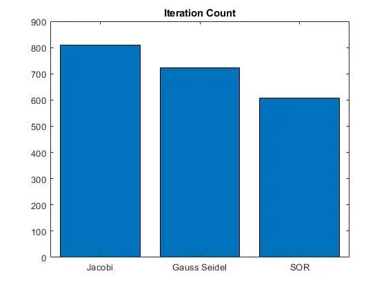
Iteration count:

Steady-state:

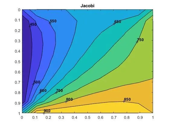
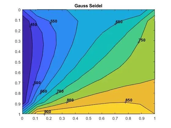
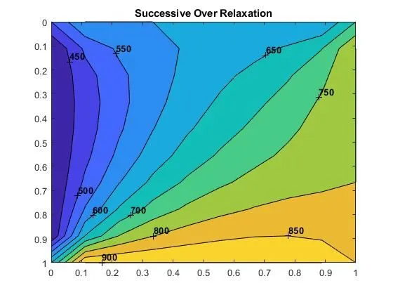
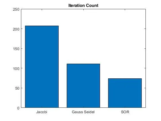
From the above results, it could be understood that the Successive over-relaxation (SOR) method took the least number of iterations to achieve convergence and it is the most time-efficient method among the three.

Transient state:

The number of iterations required to converge for the implicit scheme, the results follow a similar trend of the steady-state with Jacobi > GS > SOR in terms of the number of iterations required for convergence.

It can be concluded that the transient solution takes more iteration for convergence. Also, the transient implicit scheme is the most efficient scheme computationally as it is unconditionally stable. The principal reason for using implicit solution methods, which are more complex to program and require more computational effort in each solution step, is to allow for large time-step sizes. The transient implicit scheme can be employed for a larger time step size because of unconditional stability which lacks in case of the explicit method.