Week 5.1 - Mid term project - Solving the steady and unsteady 2D heat conduction problem
AIM:
To solve the steady and unsteady 2D heat conduction problem
CONTEXT:
- Introduction
- Governing PDE and boundary conditions
- Steady state heat conduction
- Unsteady state heat conduction
- Stability analysis
- Convergence and comparison
- Conclusion
INTRODUCTION:
TYPES OF HEAT TRANSFER:
1. Conduction: Heat transfer due to molecular interaction within a solid or stationary fluid.
Governing PDE (heat diffusion equation)
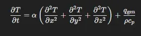
Where.
- α = k/pcp (thermal diffusivity)
- qgen (heat generation)
Application:
- cooling of electronic chips (CPU heat spreaders)
- Heat conduction in walls (insulation design)
- heat transfer in metal rod (welding and manufacturing)
2. Convection: heat transfer due to fluid motion, including advection (bulk movement of fluid) and diffusion (spreading due to molecular motion)
Governing PDE (Convection - diffusion equation)

where,
- u,v,w = velocity component (advection)
- α∇2T = heat diffusion
Application:
- cooling of air radiators (forced convection)
- Natural airflow in rooms (HVAC design)
- Heat transfer in heat exchangers (power plants)
3. Radiation: Heat transfer via infrared radiation, required no medium
Governing PDE (Radiative transfer equation - RTE)
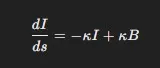
Where,
- I = radiation intensity
- K = absorption co-efficient
- B = blackbody radiation intensity
- dI/ds = radiation intensity changes along the path
Application:
- sun heating the earth
- infrared heating system (space heaters)
- thermal radiation in furnaces (high temperature processes)
4. Conjugate heat transfer (CHT): It occurs when heat conduction in solids interacts with convection in fluids and used in systems where heat moves between a solid (wall, metal) and a moving fluid
Governing PDE:
Heat conduction in the solid (Diffusion equation)
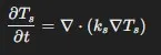
where,
- Ts = temperature in the solid
- Ks = thermal conductivity of the solid
Heat conduction in the fluid (energy equation)

where,
- Tf = Temperature in the fluid
- u,v,w = velocity component in x,y,z direction
- αf = thermal diffusivity of the fluid
Application:
- Heat sinks in electronic (cooling processors)
- cooling of gas turbine blades (thermal management)
- heat transfer in refrigeration system (efficient energy transfer)
5. Phase change (Boiling, melting, condensation):
heat transfer during a phase transition (solid - liquid - gas)
Governing PDE: (Stefan's equation for melting/ freezing)
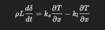
where,
- L = latent heat
- δ = moving phase boundary
- p = density
- Ks = thermal conductivity of solid
- Kl = thermal conductivity of liquid
- dt/dx = temperature gradient
Application:
- Ice melting in water (cryogenics)
- boiling in power plants (steam generation)
- condensation in refrigerators (air conditioning)
What type of heat transfer used in this project and why?
Heat conduction PDE:
- It is a mathematical equation that describes how the heat diffuses or spread through a material over time.
- It is a fundamental concept of thermodynamics and heat transfer
∂T/∂t = α * (∂2T/∂x2 + ∂2T/∂y2 + ∂2T/∂z2) - (3D transient heat conduction)
where,
T is the temperature
t is the time
α is the thermal diffusivity of the material
x,y,z are the spatial co-ordinates
Uses of heat conduction PDE in CFD:
- CFD simulation can accurately predict temperature distributions in complex systems, helping engineers optimize design for thermal performance.
- non uniform temperature distributions can lead to thermal stress, which can cause material failure, CFD helps analyze theses stresses and prevent problems
- CFD can be used to design more efficient heat exchanges, cooling systems and other thermal devices.
GOVERNING PDE AND BOUNDARY CONDITIONS:
Types of heat conduction with respect to time:
steady state
- A heat transfer process is in steady state when the temperature at all points within the system remain constant over time.
- even though heat might be flowing through the system the temperature at any specific location doesn't change
3D steady state PDE formula:
0 = (∂2T/∂x2 + ∂2T/∂y2 + ∂2T/∂z2)
where,
T is the temperature
x,y,z are the spatial co-ordinates
unsteady state
- A heat transfer process is unsteady or transient when the temperature at one or more points within the system change over time.
- the temperature distribution is evolving as the system adjusts to new conditions
3D unsteady state PDE formula:
∂T/∂t = α * (∂2T/∂x2 + ∂2T/∂y2 + ∂2T/∂z2)
where,
T is the temperature
t is the time
α is the thermal diffusivity of the material
x,y,z are the spatial co-ordinates
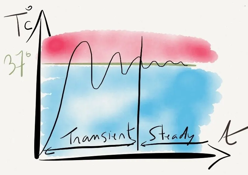
General 2nd order PDE
A * (∂2U/∂x2) + B * (∂2U/∂x∂y) + C * (∂2U/∂y2) + D * (∂U/∂x) + E * (∂U/∂Y) + G = 0
2D steady state heat conduction:
0 = (∂2T/∂x2 + ∂2T/∂y2)
PDE check: (B2 - 4AC) = 0 - 4(1)(1) = -4 <0>
therefore, it is an elliptic PDE. the solution at any point depends on the values at all surrounding points. Hence Dirichlet BC is used in the problem.
2D unsteady state heat conduction:
∂T/∂t = α * (∂2T/∂x2 + ∂2T/∂y2)
PDE check: (B2 - 4AC) = 0 - 4(-α)(-α) = -4α2 < 0>
since α (thermal diffusivity is a positive value -4α2 < 0>
The reason the unsteady heat equation is still parabolic, even though the discriminant is less than 0, is because the time derivative plays a crucial role. Hence same Dirichlet BC is used in the problem but with respect to time.
The boundary conditions for the problem are as given below:
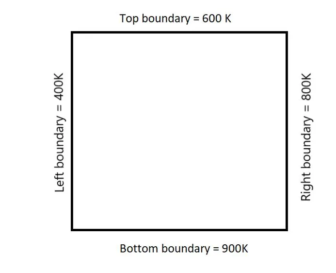
STEADY STATE HEAT CONDUCTION:
Derivation:
In steady state analysis, the initial transient temperature is omitted, and all the points are assumed to attain the equilibrium temperature. so, the temperature in the steady state does not vary with respect to time. hence the formula will be,
(∂2T/∂x2 + ∂2T/∂y2) = 0
Now we will solve the steady state equation-based on the discretization formula and derived with each of the following iterative schemes.
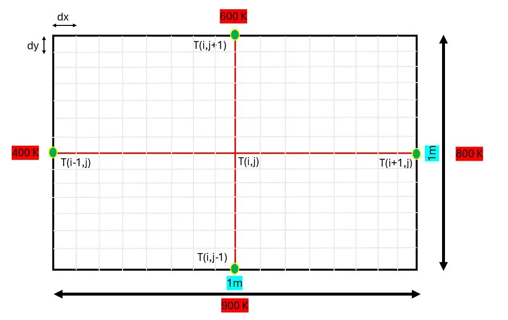
discretizing the above steady state equation using second order central difference approach we get,
[(T(i-1,j) -2*T(i,j) + T(i+1,j)) / dx2 ] + [(T(i,j-1) -2*T(i,j) + T(i,j+1)) / dy2 ] = 0
(2*T(i,j)/dx2) + (2*T(i,j)/dy2) = [(T(i-1,j) + T(i+1,j))/dx2] + [(T(i,j-1) + T(i,j+1))/dy2]
where,
K = T(i,j) * [(2*(dx2 + dy2)) / dx2 * dy2]
(1.1) Gauss Jacobi scheme:
let i denotes the ith row and j denotes the jth column. then T(i,j) denotes the temperature at the node placed at ith row and jth column. now we will rewrite the discretization formula based on the indices considered as
Tq+1(i,j) = 1/K * {[(Tq(i-1,j) + Tq(i+1,j))/dx2] + [(Tq(i,j-1) + Tq(i,j+1))/dy2]}
- T(i,j) is the temperature in the present state
- T(i-1,j) is the temperature in the left boundary
- T(i+1,j) is the temperature in the right boundary
- T(i,j-1) is the temperature in the bottom boundary
- T(i,j+1) is the temperature in the top boundary
- dx and dy are the distance between each node.
In gauss Jacobi scheme, we will find the value of given node say T(i,j) at q+1 iteration by considering the pervious iteration values (qth iteration) of the neighboring nodes.
after that we solve the above formula for each node and find the solution by iteration until Tq(i,j) - Tq+1(i,j) <= 1e-4
(1.2) Gauss seidel scheme:
In this scheme, we find the value of the give node, say T(i,j) at q+1 iteration by considering the previous iteration values of neighboring nodes from q+1 iteration and unknow neighboring values from the previous iteration (qth iteration)
{Tq+1(i,j)}Gauss = 1/K * {[(Tq+1(i-1,j) + Tq(i+1,j))/dx2] + [(Tq+1(i,j-1) + Tq(i,j+1))/dy2]}
after than we will iterate until the tolerance of 1e-4 is achieved.
(1.3) successive relaxation scheme:
In successive relaxation scheme, we extrapolate the gauss seidel method for faster or step further. It introduces a relaxation factor that controls how much the solution is updated in each iteration.
Over relaxation (ω>1) if the relaxation factor is greater than 1, it overshoots the correction, it overshoots the correction, meaning makes a larger adjustment to the variable than gauss seidel method would. this can help accelerate convergence.
Under relaxation (ω<1> if the relaxation factor is less than 1, it undershoots the correction making a smaller adjustment. this can be useful if the gauss seidel method is diverging or oscillating
{Tq+1(i,j)}SOR = (1-ω) * Tq(i,j) + ω * {Tq+1(i,j)}Gauss
we iterate the same until the tolerance of 1e-4 is achieved.
Matlab code: (Steady state 2D heat conduction)
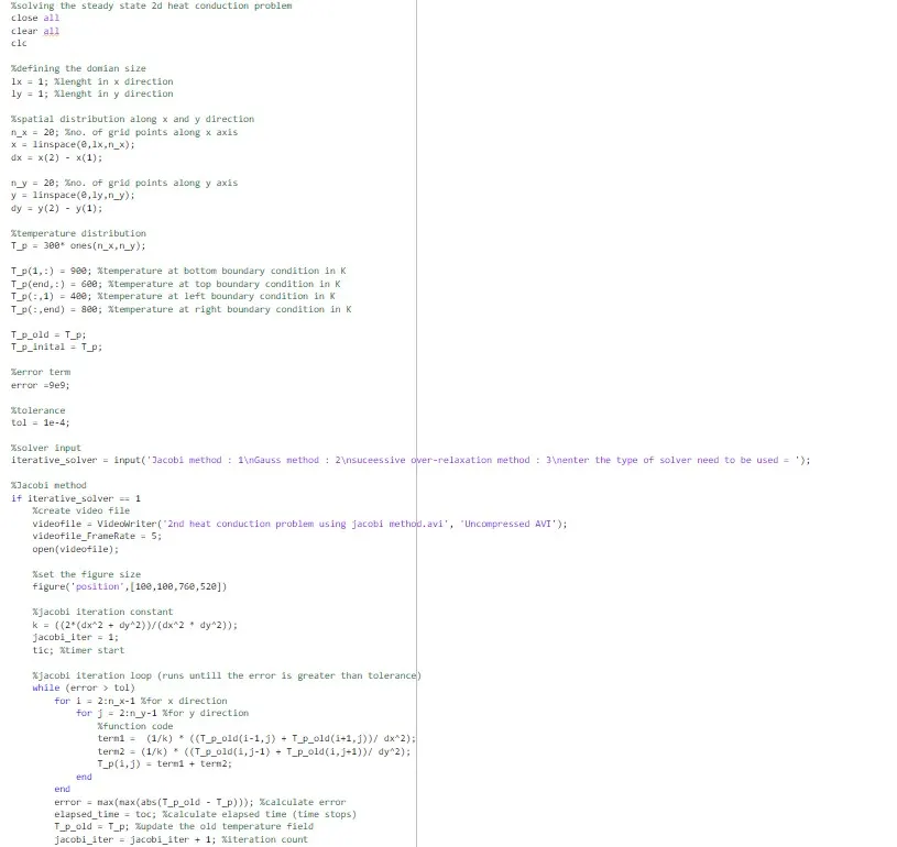
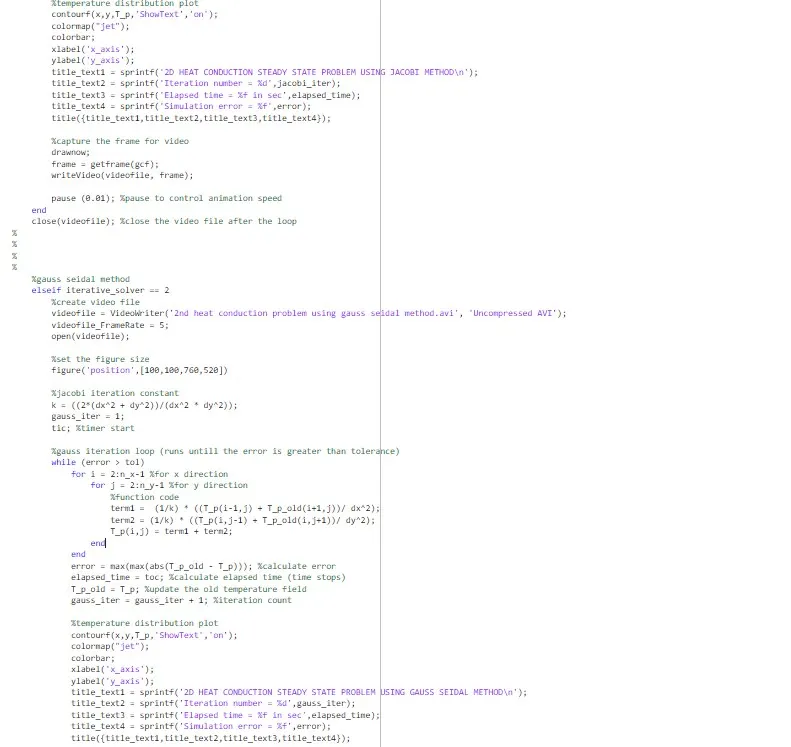
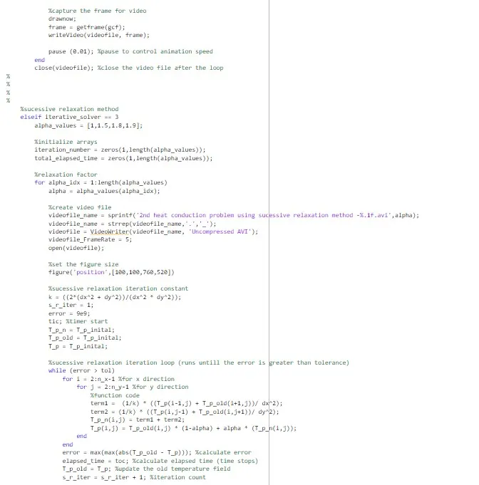
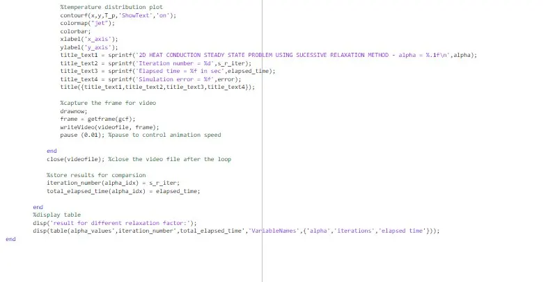
Code explanation:
Initialization:
- lx, ly : define the length of the square domain in the x and y direction
- n_x , n_y: number of grid points in the x and y direction
- x,y: create the x and y co-ordinate vectors using linspace
- dx,dy: calculate the grid spacing
- T_P: initialize the temperature matrix. its initially filled with 300k
- Boundary conditions: the code sets the temperature on the boundaries of the square
- Bottom: 900K
- Top: 600K
- left: 400K
- Right: 800K
- T_p_old: stores the temperature from the previous iteration
- T_p_initail: stores the initial temperature distribution
- error, Tol: initiate the error and tolerance for convergence.
- iterative solver: prompts the user to choose which method to use (1 for Jacobi, 2 for gauss-seidel, 3 for successive relaxation)
Jacobi method: (if iterative solver == 1)
- video creation: sets up a video file to store the animation of the temperature distribution.
- iteration loop: the while (error>Tol) loop continues until the error falls below the tolerance
- Jacobi update: inside the loop the code calculates the temperature at each interior point (i,j) using the Jacobi formula:
T_p(i,j) = (1/k) * [(T_p_old(i-1,j) + T_p_old(i+1,j))/dx^2] + (1/k) * [(T_p_old(i,j-1) + T_p_old(i,j+1))/dy^2];
- note that old temperature values (T_p_old) are used to calculate the new temperature values (T_p)
- error calculation: calculate the maximum difference between the old and new temperature matrices.
- update T_p_old: copies the new temperature matrix to the old temperature for the next iteration.
- plotting: creates a contour plot of the temperature distribution and adds titles with iteration, number, elapsed time and error
- video frame capture: captures the current plot as a frame and adds to the video.
Gauss-seidel method: (if iterative solver == 2)
- this section is very similar to the Jacobi method. the key difference is in the temperature update:
T_p(i,j) = (1/k) * [(T_p(i-1,j) + T_p_old(i+1,j))/dx^2] + (1/k) * [(T_p(i,j-1) + T_p_old(i,j+1))/dy^2];
- notice that it uses (T_p(i-1,j) and T_p(i,j-1), which are the updated values from the current iteration =, unlike the Jacobi method. this is what makes it gauss seidel method.
Successive relaxation method: (if iterative solver == 3)
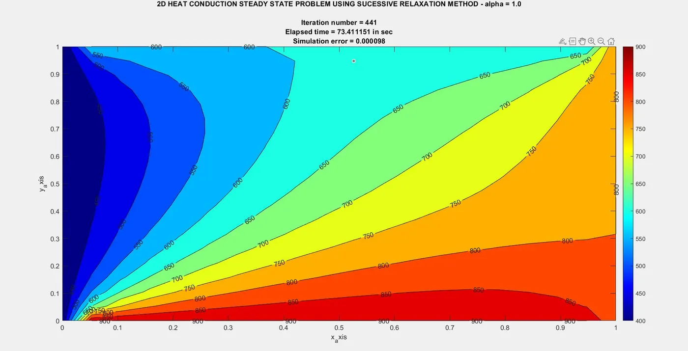
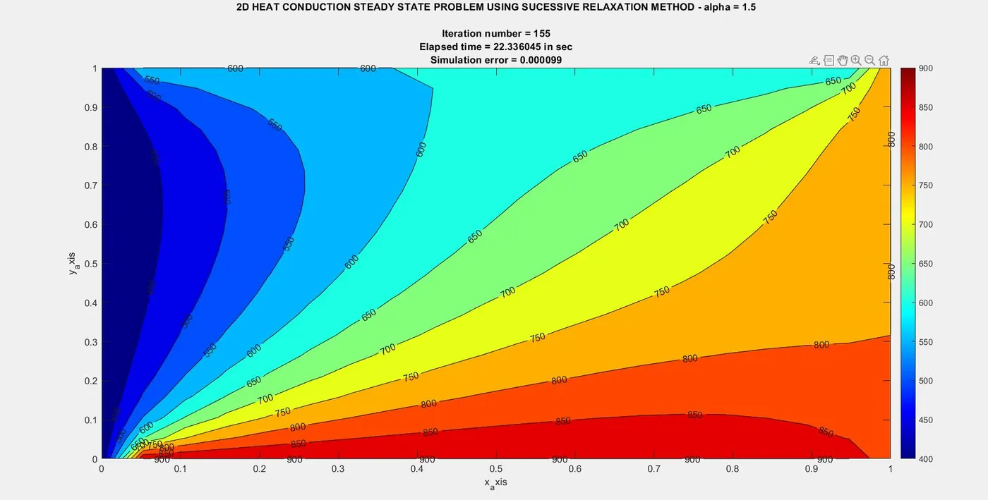
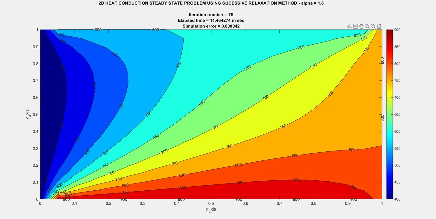
- relaxation over factor (alpha or omega): this code tests several values of alpha (1,1.5,1.8,1.9). this is the key parameter of SOR.
- SOR update: the temperature upade is
T_p_n(i,j) = (1/k) * [(T_p(i-1,j) + T_p_old(i+1,j))/dx^2] + (1/k) * [(T_p(i,j-1) + T_p_old(i,j+1))/dy^2];
T_p(i,j) = T_p_old(i,j) * (1-alpha) + alpha * (T_p_n(i,j));
- here T_p_n is an intermediate value. the final temperature T_p(i,j) is a weighted average of the old temperature and newly calculate temperature.
- alpha > 1 is over relaxation
- Result comparison: the code stores the number of iterations and elapsed time for each value of alpha and displays them in a table at the end. this allows you to see how different relaxation factor affect convergence.
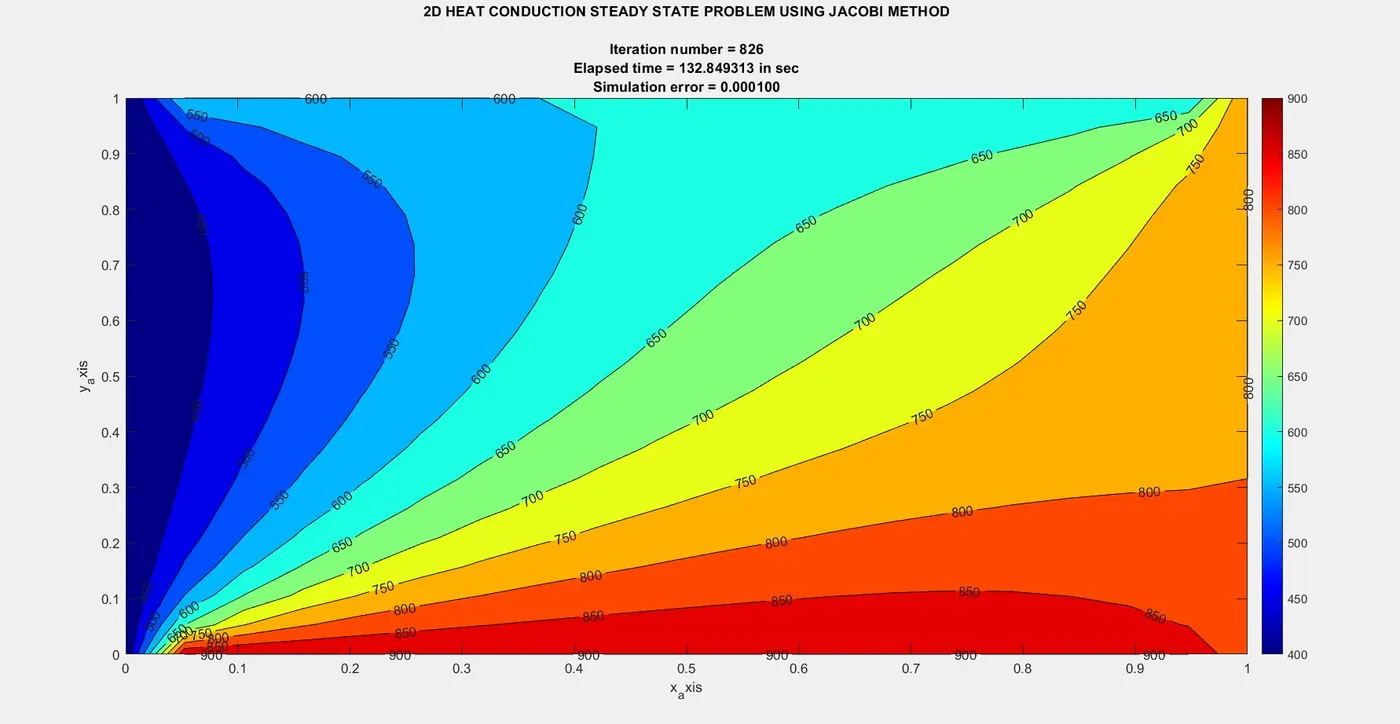
Result plotting:
Jacobi method
Gauss seidel method:
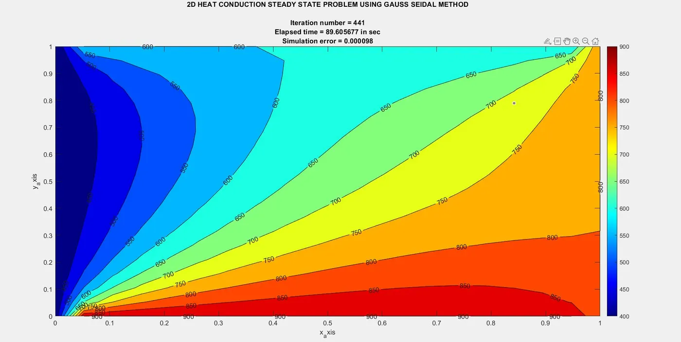
Successive over relaxation method: (alpha - 1.0)
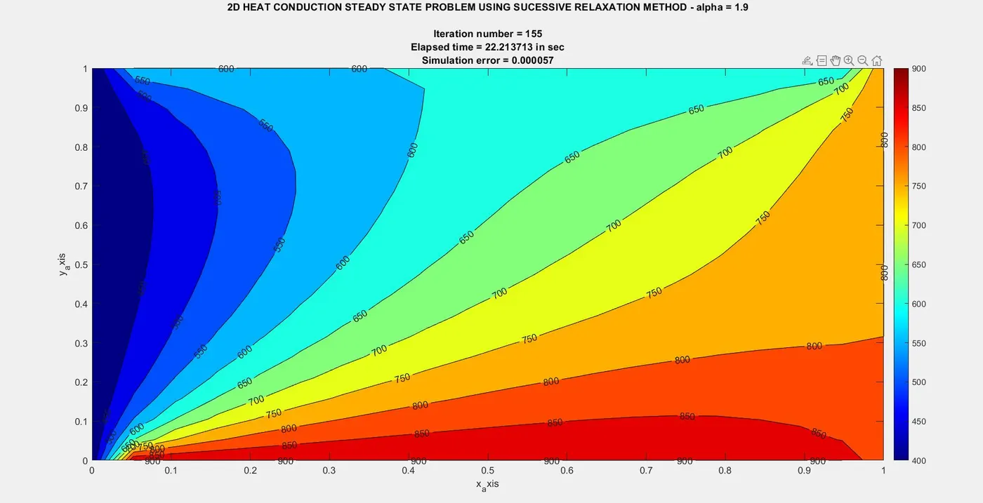
Successive over relaxation method: (alpha - 1.5)
Successive over relaxation method: (alpha - 1.8)
Successive over relaxation method: (alpha - 1.9)
SOR comparison table:
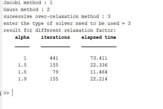
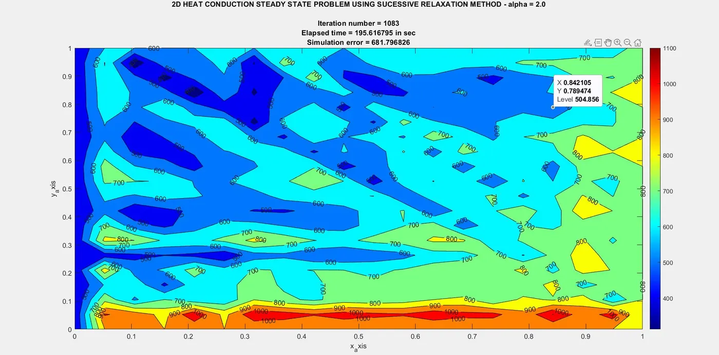
- when the relaxation factor in SOR method is too high (like above 1.9), the solution tends to diverge the method overcorrects too aggressively in each iteration
- SOR aims to accelerate convergence by taking larger steps towards the solution than gauss seidel method. the relaxation factor controls the size of these steps
- when α>1.9 in this case, the method "overshoots" the correction. instead of just moving closer to the solution in each iteration, it moves past the solution sometimes significantly.
- It depends on factor like the size of the grid (dx,dy) the boundary conditions and nature of the equation being solved.
- for this particular problem setup, 1.9 seems to be roughly the upper limit where the overcorrection becomes too much causing the solution to diverge.
- on other hand, if α is too small (under relaxation) the method becomes very slow. it takes tiny cautious steps towards the solution, so it takes many more iterations to converge.
Steady state result analysis:
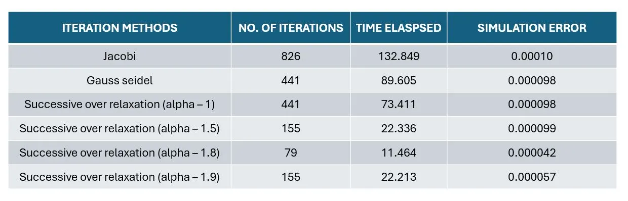
Thus, as far from the table, we have analyzed different iterations for steady state method to find the better iterative solver. the successive over relaxation method with alpha value of 1.8 is given much better results while compared to other iteration methods which has converged within 79 iteration and its time taken is 11.464 sec.
UNSTEADY STATE HEAT CONDUCTION:
- Also known as transient heat conduction, describes the process where temperature within an object or system change over time.
- This is in contrast to steady state heat conduction, where temperature remain constant.
∂T/∂t = α * (∂2T/∂x2 + ∂2T/∂y2)
This transient analysis has two types,
- Implicit
- explicit
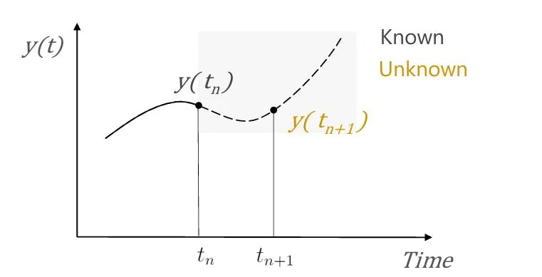
Explicit solver:
Time stepping: solves the equation using the known information from the previous time step
computation cost: low per time step
stability: conditioned by CFL condition, meaning smaller steps are required for stability.
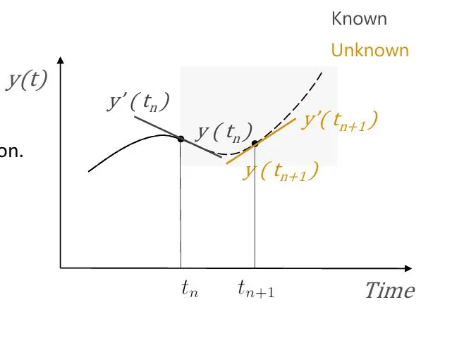
Implicit solver:
Time stepping: solves the equations by considering unknowns at the next time step
computational cost: high per time step
memory requirement: high
stability: unconditionally stable, meaning larger time steps can be used.
Explicit unsteady state heat conduction:
- An explicit method for solving a differential equation is numerical procedure where the solution at the next time step (tn+1) is calculate exclusively using known quantities at the current time step (tn)
- from the above 2d heat conduction unsteady state PDE, it needs to discretize to central differencing scheme to solve the problem
(Tn+1(i,j) / dt) - α * [(T(i-1,j) -2*T(i,j) + T(i+1,j)) / dx2 ] + [(T(i,j-1) -2*T(i,j) + T(i,j+1)) / dy2 ]
Tn+1(i,j) = Tn(i,j) + α * dt * [(Tn(i-1,j) -2*Tn(i,j) + Tn(i+1,j)) / dx2 ] + [(Tn(i,j-1) -2*Tn(i,j) + Tn(i,j+1)) / dy2 ]
- This is the explicit form at time level - n
- In a CFD simulation, the Courant number broadly indicates how much the information travels (u) across a computational grid cell (dh) in a unit of time (dt).
- If the Courant number is greater than one, it means that the information propagates through more than one grid cell at each time step, making the solution inaccurate and potentially leading to nonphysical results or divergence of the solution in certain integration schemes.
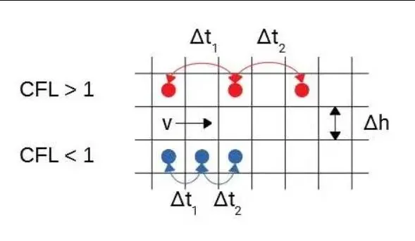
- for the 2D heat conduction,
CFL NO. = α*dt*(1/dx2 + 1/dy2) <= 0.5
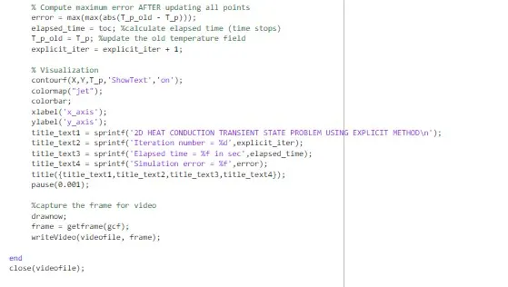
Matlab code: (Explicit unsteady state heat conduction)
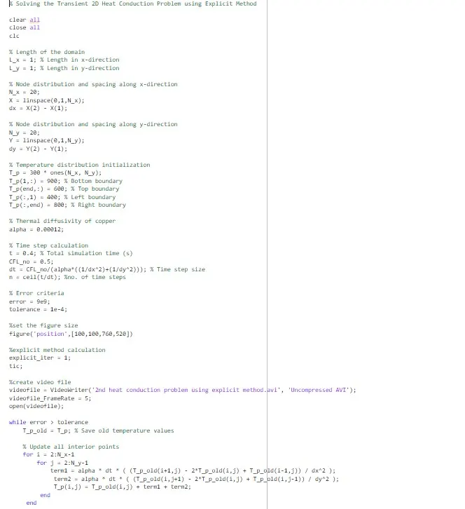
Code explanation:
- This code is same as the steady state 2D heat conduction program, but the only difference is the introducing the time variable
- the von Newmann stability analysis is commonly used to determine the stability limit for explicit methods for the 2d heat equation, the stability criterion will be
- CFL NO. = α*dt*(1/dx2 + 1/dy2) <= 0.5
- from this we can find the time step size for each iteration.
- if we increase the CFL no above 0.5, the instability will occur.
- hence, we set the CFL at max condition and find the dt according to the value
- the code will be run until the tolerance of 1e-4 is reached
- Explicit update: inside the loop the code calculates the temperature at each interior point (i,j) with respect to the time step.
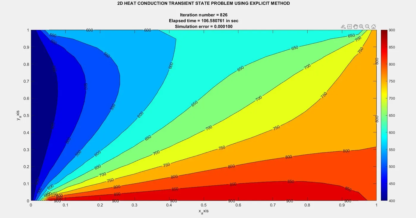
Result plotting:
Implicit unsteady state heat conduction:
An implicit method is a numerical procedure where the solution at the next time step (tn+1) is defined implicitly by an equation that involves the unknown solution at the next time step itself as well as know quantities at the current time step (tn)
Tn+1(i,j) = Tn(i,j) + α * dt * [(Tn+1(i-1,j) -2*Tn+1(i,j) + Tn+1(i+1,j)) / dx2 ] + [(Tn+1(i,j-1) -2*Tn+1(i,j) + Tn+1(i,j+1)) / dy2 ]
where,
K1 = (α * dt) / dx2
K2 = (α * dt) / dy2
By re arranging the equation we get,
Tn+1(i,j) = Tn(i,j) + K1 (Tn+1(i-1,j) + Tn+1(i+1,j) ) + K2 (Tn+1(i,j-1) + Tn+1(i,j+1) )
So, this is the implicit form equation to calculate unknow temperature at the next time step
Implicit methods require solving a system of equations at each time step.
Iterative solvers (Jacobi, Gauss-Seidel, SOR) are efficient ways to do this.
Explicit methods calculate temperatures directly, so there's no system of equations and iterative solvers are unnecessary.
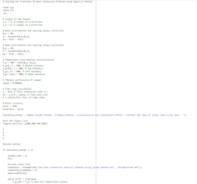
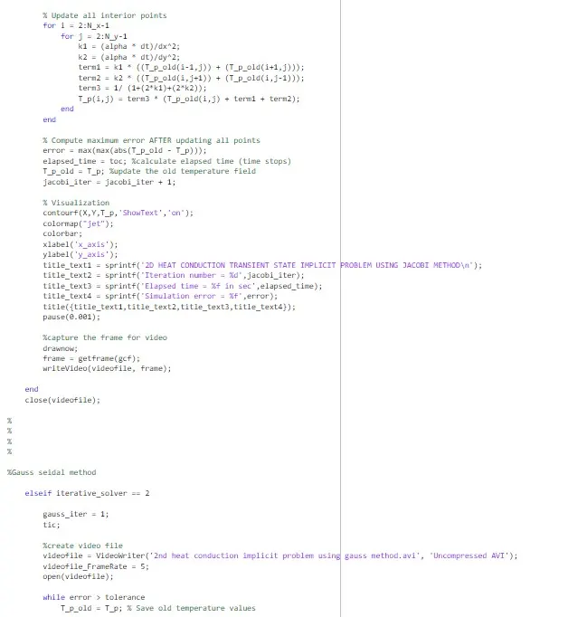
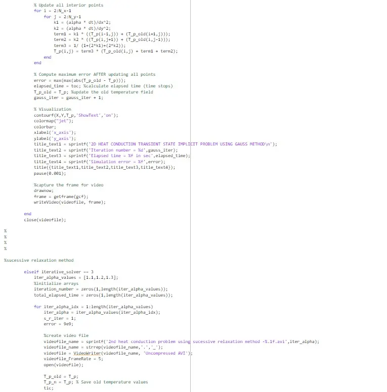
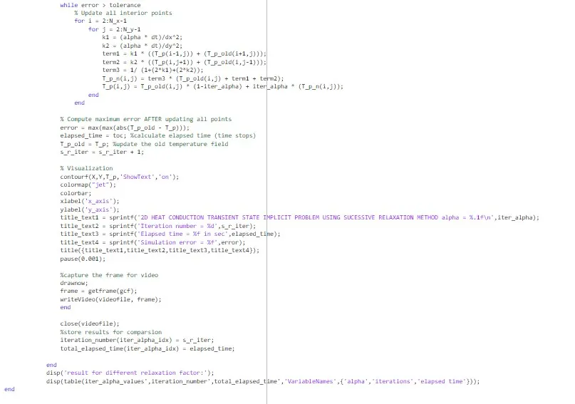
Matlab code: (implicit unsteady state heat conduction)
Code explanation:
- Domain: Square 2D region discretized into a grid.
- Boundary Conditions: Fixed temperatures specified at the edges of the square.
- Time Stepping: Calculates temperatures at discrete time steps, advancing until a final time.
- For implicit methods (backward Euler, crank Nickolson), the time step stability is typically unconditional meaning we can choose relatively large time steps without violating stability.
- hence the maximum implicit time step can be approximated using characteristic time scale.
- dt(max) = L2/α
- Implicit Nature: Solves a system of equations at each time step to determine future temperatures. This is necessary for stability.
- Iterative Solvers: Employs iterative methods (Jacobi, Gauss-Seidel, SOR) to solve the system of equations at each time step.
- SOR (Successive Over-Relaxation): Uses a relaxation factor to potentially accelerate convergence, and tests different relaxation factor values to find the best one.
- Visualization: Creates a video showing the temperature distribution evolving over time.
- Performance Comparison: Compares the different methods (and SOR relaxation factors) based on iterations and computation time.
- Output: Video of temperature distribution and a table comparing solver performance.
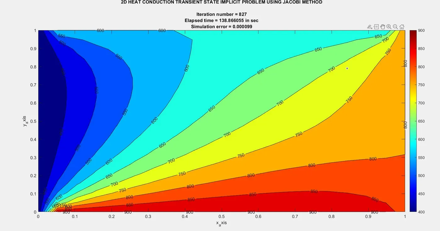
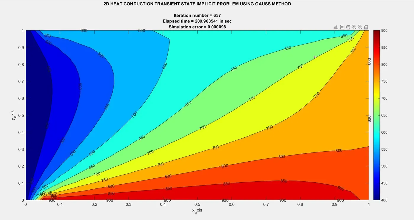
Result Plotting:
Jacobi method
Gauss seidel method:
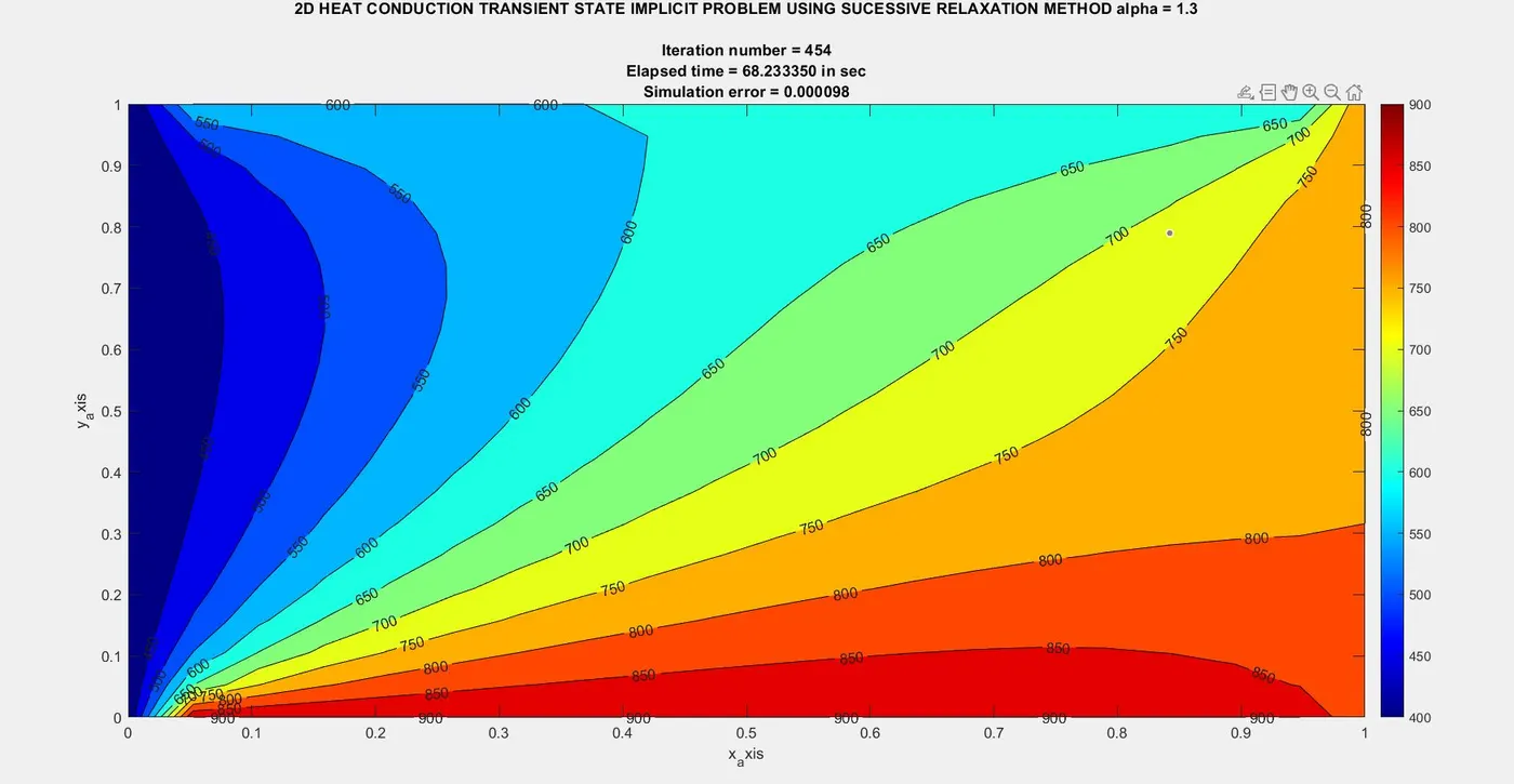
SOR method: alpha - 1.3
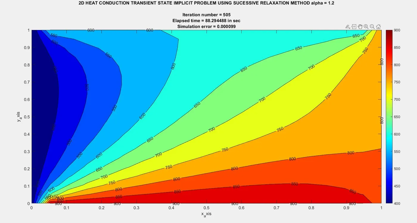
SOR method: alpha - 1.2
SOR method: alpha - 1.4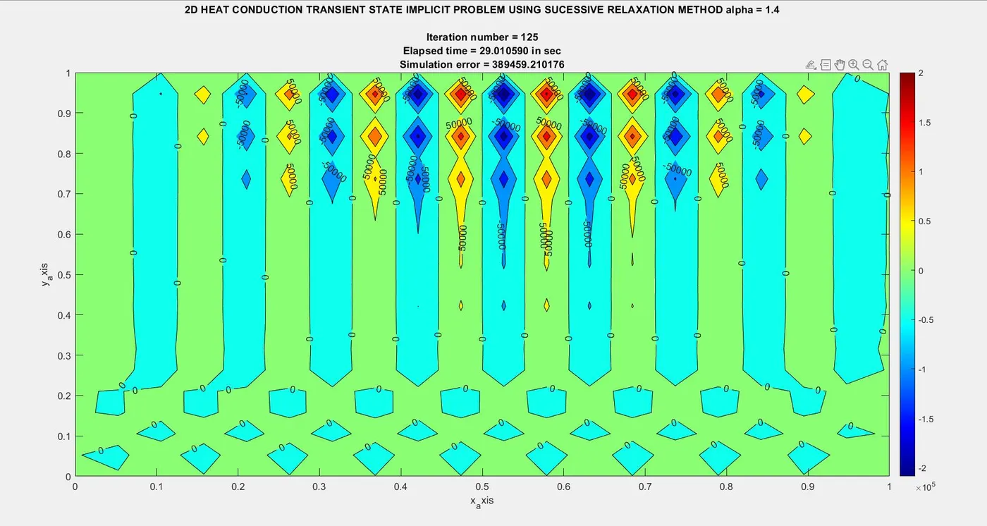
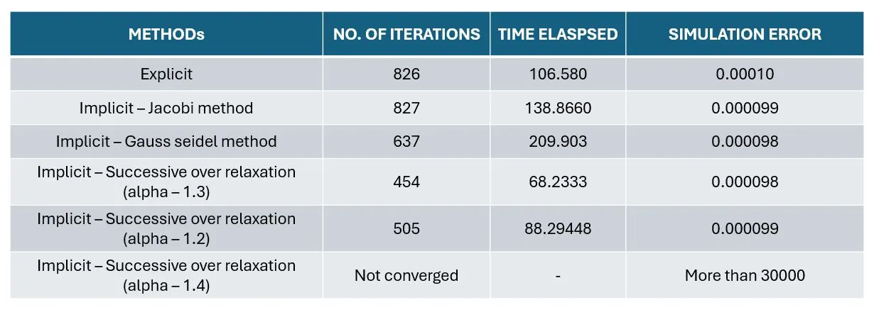
Result comparison table:
Result conclusion (Unsteady state)
Explicit method:
Disadvantages:
- stability depends on small dt (CFL condition)
- slow convergence for long term simulations due to small time steps
When to use:
- short term simulations
- fast changing dynamics
- when memory or computational resource are limited.
Implicit method:
Advantages:
- unconditionally stable, allowing larger time steps
- faster convergence for long term or steady state problems
- better for stiff problem (e.g. diffusion)
- higher accuracy with larger time steps
Disadvantages:
- High computational cost per step (requires solving system of equation)
- higher memory usage due to storage of matrices
- more complex to implement
When to use:
- long term simulations or steady state problems
- slow diffusive process or stiff problems
- when stability over time is critical.
Instability in implicitly SOR - alpha (1.3 above)
- so, from the table, if we increase the alpha value above 1.3 in implicit SOR it will be having divergence issue.
- this is because the adjustment to each point is too large, for problems where heat conduction is not changing drastically. this large adjustment can create oscillations or divergence in solution.
- hence this leads to overshooting where the temperature values may jump too far in each iterations causing instability