Week 5.1 - Mid term project - Solving the steady and unsteady 2D heat conduction problem
*AIM:-
To solve the 2D heat condution equation using a steady state solver and transient solver using interative techniques.
*Introdution:-
-The 2D heat condution equation is:-
`(∂T)/(∂t)-α((∂^2 T)/(∂x^2) +(∂^2 T)/(∂y^2) )=0`
*Derivation for steady state:-
-There is no change of fluid property with respect to time is called steady state condition.
`(∂^2 T)/(∂x^2) +(∂^2 T)/(∂y^2) =0`
-There are three methods are available for solve this equation numerically:-
i) Jacobi method
ii) gauss seidel method
iii) succesive over relaxation method (SOR)
Note:- There are two second order terms available in the equation, so for discretize that using the central difference sceme.
`(T_L-2T_p+T_R)/(∆x^2) +(T_T-2T_p+T_B)/(∆y^2) =0`
Where, `T_L=T_((i-1,j)`
`T_R=T_((i+1,j)`
`T_T=T_((i,j-1)`
`T_B=T_((i,j+1)`
`T_p=T_((i,j)`
`(2T_p)/(∆x^2 )+(2T_p)/(∆y^2) =(T_L+T_R)/(∆x^2) +(T_T+T_B)/(∆y^2)`
`T_p ((2(∆x^2+∆y^2))/(∆x^2 ∆y^2 ))=(T_L+T_R)/(∆x^2) +(T_T+T_B)/(∆y^2)`
-Here, we assume
`k= (∆x^2 ∆y^2)/(2(∆x^2+∆y^2))`
`T_p×k=(T_L+T_R)/(∆x^2) +(T_T+T_B)/(∆y^2)`
`T_p=1/k[(T_L+T_R)/(∆x^2) +(T_T+T_B)/(∆y^2) ]`
i) For jacobi:-
`T_p^(n+1)=1/k[(T_L+T_R)/(∆x^2) +(T_T+T_B)/(∆y^2) ]^n`
ii) For gauss seidel:-
`T_p^(n+1)=1/k[(T_L+T_R)/(∆x^2) +(T_T+T_B)/(∆y^2) ]^(n+1)`
iii) For SOR:-
`T_p^(n+1)=(1-α)T_p^n+α/k[(T_L+T_R)/(∆x^2) +(T_T+T_B)/(∆y)^2 ]^(n+1)`
Here, `α`=Relaxation factor
*Initial condition:-
*Absolute error criteria= 1e-4
*Boundary condition:-
-Top Boundary = 600 K
-Bottom Boundary = 900 K
-Left Boundary = 400 K
-Right Boundary = 800 K
* nx=ny (Number of grid point along x-direction is equal to number of grid point along y direction)
*Explaination of program:-
-First of all open the octave software and open the new script.
-First three lines is as ussual. Its use for clear all thing in the work space and command window.
-Then discrite the domain in to x and y direction. Here we provide 10 discrite points.
-Then provide initial condition just like temperature for the every boundary and at the corners. Also provide the temperatu for every grid points.
-Then provide error and tolerance.
-After that use while function for reach to our criteria.
-Then use counter plot for see the result in the plot.
i) Matlab code for jacobi method:-
clear all
close all
clc

%number of grid point in x and y direction
nx=10;
ny=nx;

%discretize domain in x and y direction
x=linspace(0,1,nx);
y=linspace(0,1,ny);

%distance between  two nearly nodes in x and y direction respectively
dx=x(2)-x(1);
dy=y(2)-y(1);

%initial temperature
T=300*ones(nx,ny);
%Boundary temperature
T(:,1)=400; %Tleft=400k
T(1,:)=600; %Ttop=600k
T(:,end)=800;  %Tright=800k
T(end,:)=900;  %Tbottom=900k

%temperature at the corner
T(1,1)=(600+400)/2;
T(1,nx)=(600+800)/2;
T(end,1)=(400+900)/2;
T(end,end)=(900+800)/2;


k=2*((dx^2)+(dy^2))/((dx^2)*(dy^2));

error=1e9;
tol=1e-4
Told=T;
jacobi_iter=1
interative_solver=1
if interative_solver==1
  while (error>tol)
    for i=2:(nx-1)
      for j=2:(ny-1)
           T(i,j)=(1/k)*(((Told(i-1,j)+Told(i+1,j))/dx^2)+((Told(i,j-1)+Told(i,j+1))/dy^2));
      endfor
    endfor
    error=max(max(abs(T-Told)));
    Told=T;
    jacobi_iter=jacobi_iter+1;
  endwhile
  figure(1)
  [a,b]=contourf(x,y,T);
  set(gca,'YDIR','reverse');
  clabel(a,b);
  colormap(jet);
  colorbar;
  text=sprintf('number of jacobi interation:%d',jacobi_iter);
  title(text,'color','r');
  xlabel('width');
  ylabel('height');
  xticks(0:0.1:1);
  yticks(0:0.1:1);
endif
ii) Matlab code for gauss seidel method:-
clear all
close all
clc

nx=10;
ny=nx;

x=linspace(0,1,nx);
y=linspace(0,1,ny);

dx=x(2)-x(1);
dy=y(2)-y(1);

T=300*ones(nx,ny);

T(:,1)=400; %Tleft=400k
T(1,:)=600; %Ttop=600k
T(:,end)=800;  %Tright=800k
T(end,:)=900;  %Tbottom=900k

T(1,1)=(600+400)/2;
T(1,nx)=(600+800)/2;
T(end,1)=(400+900)/2;
T(end,end)=(900+800)/2;


k=2*((dx^2)+(dy^2))/((dx^2)*(dy^2));

error=1e9;
tol=1e-4
Told=T;
gs_iter=1
interative_solver=2
if interative_solver==2
  while (error>tol)
    for i=2:(nx-1)
      for j=2:(ny-1)
           T(i,j)=(1/k)*(((T(i-1,j)+Told(i+1,j))/dx^2)+((T(i,j-1)+Told(i,j+1))/dy^2));
      endfor
    endfor
    error=max(max(abs(T-Told)));
    Told=T;
    gs_iter=gs_iter+1;
  endwhile
  figure(1)
  [a,b]=contourf(x,y,T);
  set(gca,'YDIR','reverse');
  clabel(a,b);
  colormap(jet);
  colorbar;
  text=sprintf('number of gs interation:%d',gs_iter);
  title(text,'color','r');
  xlabel('width');
  ylabel('height');
  xticks(0:0.1:1);
  yticks(0:0.1:1);
endif
iii) Matlab code for SOR method:-
clear all
close all
clc

nx=10;
ny=nx;

x=linspace(0,1,nx);
y=linspace(0,1,ny);

dx=x(2)-x(1);
dy=y(2)-y(1);

T=300*ones(nx,ny);

T(:,1)=400; %Tleft=400k
T(1,:)=600; %Ttop=600k
T(:,end)=800;  %Tright=800k
T(end,:)=900;  %Tbottom=900k

T(1,1)=(600+400)/2;
T(1,nx)=(600+800)/2;
T(end,1)=(400+900)/2;
T(end,end)=(900+800)/2;


k=2*((dx^2)+(dy^2))/((dx^2)*(dy^2));

error=1e9;
tol=1e-4;
Told=T;
w=1.25;
sor_iter=1
interative_solver=3
if interative_solver==3
 while (error>tol)
    for i=2:nx-1
      for j=2:ny-1
            term_1=(T(i-1,j)+Told(i+1,j))/(k*dx^2);
            term_2=(T(i,j-1)+Told(i,j+1))/(k*dy^2) ;
            T(i,j)=((1-w)*Told(i,j))+(w*(term_1+term_2));
      endfor
    endfor
    error=max(max(abs(T-Told)));
    Told=T;
    sor_iter=sor_iter+1;
 endwhile

 figure(1)
 [a,b]=contourf(x,y,T);
 set(gca,'YDIR','reverse');
 clabel(a,b);
 colormap(jet);
 colorbar;
 text=sprintf('number of sor interation:%d',sor_iter);
 title(text,'color','r');
 xlabel('width');
 ylabel('height');
 xticks(0:0.1:1);
 yticks(0:0.1:1);
endif
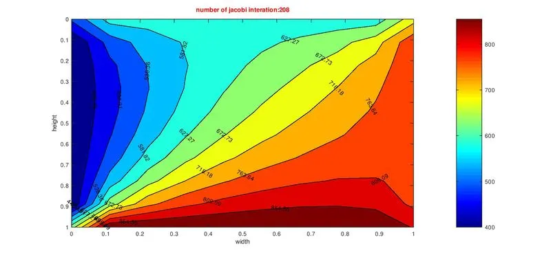
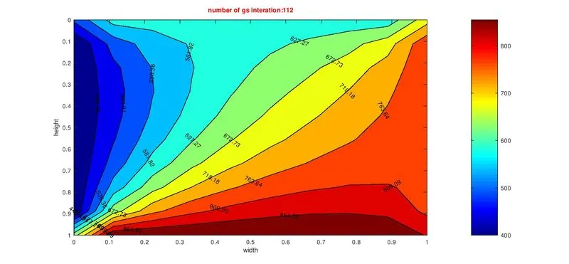
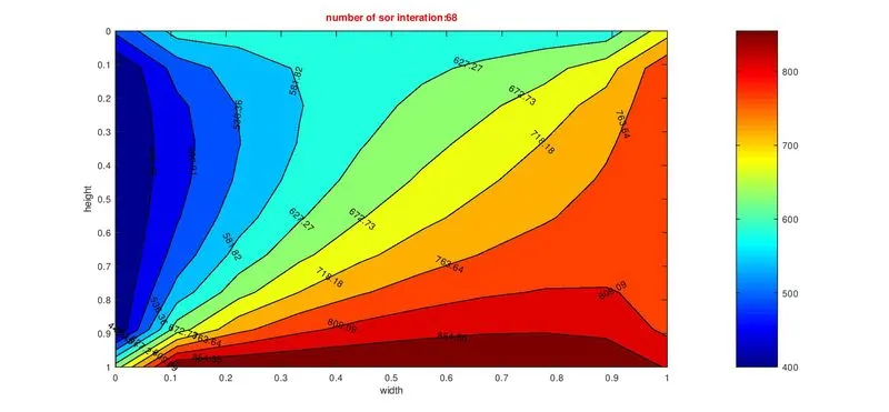
*Result of steady state analysis:-
i) Jacobi method:-
ii) Gauss seidel method:-
iii) SOR method:-
*Unsteady state 2D heat transfer:-
-There is change of fluid property with respect to time is called unsteady state condition.
-The 2D heat condution equation for unsteady is:-
`(∂T)/(∂t)-α((∂^2 T)/(∂x^2) +(∂^2 T)/(∂y^2) )=0`
Then
`(∂T)/(∂t)=α((∂^2 T)/(∂x^2) +(∂^2 T)/(∂y^2) )`
-There are three implicit methods are available for solve this equation numerically:-
i) Jacobi method
ii) gauss seidel method
iii) succesive over relaxation method (SOR)
Note:- There are two second order terms available in the equation, so for discretize that using the central difference sceme. Also in this equation time derivative term available. It means with time properties of the system is change. So obviously this is a unsteady state condition.
`(T_p^(n+1)-T_p^n)/(∆t)=α((T_L-2T_p+T_R)/(∆x^2 )+(T_T-2T_p+T_B)/(∆y^2 ))`
-We assume,
`k_1= (α×∆t)/(∆x^2 )` and `k_2= (α×∆t)/(∆y^2 )`
`T_p^(n+1)=T_p^n+k_1×(T_L-2T_p+T_R)+k_2×(T_T-2T_p+T_B)`
`T_p^(n+1)=T_p^n+k_1×(T_L^(n+1)-2T_p^(n+1)+T_R^(n+1))+k_2×(T_T^(n+1)-2T_p^(n+1)+T_B^(n+1))`
`T_p^(n+1) -k_1 T_L^(n+1)+2k_1 T_p^(n+1) -k_1 T_R^(n+1)-k_2 T_T^(n+1)+2k_2 T_p^(n+1)-k_2 T_B^(n+1)=T_p^n`
`(1+2k_1+2k_2)T_p^(n+1) -k_1 T_L^(n+1) -k_1 T_R^(n+1)-k_2 T_T^(n+1)-k_2 T_B^(n+1)=T_p^n`
`(1+2k_1+2k_2)T_p^(n+1) =T_p^n+k_1 T_L^(n+1) +k_1 T_R^(n+1)+k_2 T_T^(n+1)-k_2 T_B^(n+1)`
`T_p^(n+1) =(1/(1+2k_1+2k_2))*(T_p^n+k_1 T_L^(n+1) +k_1 T_R^(n+1)+k_2 T_T^(n+1)-k_2 T_B^(n+1))`
i) Matlab code for jacobi method:-
clear all
close all
clc

%number of grid point in x and y direction
nx=10;
ny=nx;

%discretize domain in x and y direction
x=linspace(0,1,nx);
y=linspace(0,1,ny);

%distance between  two nearly nodes in x and y direction respectively
dx=x(2)-x(1);
dy=y(2)-y(1);

%initial temperature
T=300*ones(nx,ny);
%Boundary temperature
T(:,1)=400; %Tleft=400k
T(1,:)=600; %Ttop=600k
T(:,end)=800;  %Tright=800k
T(end,:)=900;  %Tbottom=900k

%temperature at the corner
T(1,1)=(600+400)/2;
T(1,end)=(600+800)/2;
T(end,1)=(400+900)/2;
T(end,end)=(900+800)/2;

error=1e9;
tol=1e-4
Told=T;
T_prev=T;
t=1500;
dt=20;
nt=t/dt;
alpha=0.05;
k1=alpha*(dt)/(dx^2);
k2=alpha*(dt)/(dy^2);
jacobi_iter=1
time_step=1
interative_solver=1
tic;
if interative_solver==1
  for k=1:nt
     while (error>tol)
         for i=2:(nx-1)
           for j=2:(ny-1)
               term1=(1+(2*k1)+(2*k2))^(-1);
               term2=k1*term1;
               term3=k2*term1;
               h=(Told(i-1,j)+Told(i+1,j));
               v=(Told(i,j-1)+Told(i,j+1));
               T(i,j)=(T_prev(i,j)*term1)+(h*term2)+(v*term3);
          endfor
         endfor
         error=max(max(abs(Told-T)));
         Told=T;
         jacobi_iter=jacobi_iter+1;
      endwhile
      T_prev=T;
      time_step=time_step+1;
    endfor
    j_time=toc;
   figure(1)
   [a,b]=contourf(x,y,T);
   set(gca,'YDIR','reverse');
   clabel(a,b);
   colormap(jet);
   colorbar;
   title_text1=sprintf('transient implicit analysis');
   title_text2=sprintf('number of jacobi interation:%d',jacobi_iter);
   title_text3=sprintf('excution time:%f',j_time);
   title({title_text1,title_text2,title_text3});
   pause(0.04);
   xlabel('width');
   ylabel('height');
   xticks(0:0.1:1);
   yticks(0:0.1:1);
endif
ii) Matlab code for gauss seidel method:-
clear all
close all
clc

%number of grid point in x and y direction
nx=10;
ny=nx;

%discretize domain in x and y direction
x=linspace(0,1,nx);
y=linspace(0,1,ny);

%distance between  two nearly nodes in x and y direction respectively
dx=x(2)-x(1);
dy=y(2)-y(1);

%initial temperature
T=300*ones(nx,ny);
%Boundary temperature
T(:,1)=400; %Tleft=400k
T(1,:)=600; %Ttop=600k
T(:,end)=800;  %Tright=800k
T(end,:)=900;  %Tbottom=900k

%temperature at the corner
T(1,1)=(600+400)/2;
T(1,nx)=(600+800)/2;
T(end,1)=(400+900)/2;
T(end,end)=(900+800)/2;

error=1e9;
tol=1e-4
Told=T;
T_prev=T;
t=1500;
dt=20;
nt=t/dt;
alpha=0.05;
k1=alpha*(dt)/(dx^2);
k2=alpha*(dt)/(dy^2);
gs_iter=1
interative_solver=2
tic;
if interative_solver==2
  for k=1:nt
     while (error>tol)
         for i=2:(nx-1)
           for j=2:(ny-1)
               term1=(1+(2*k1)+(2*k2))^(-1);
               term2=k1*term1;
               term3=k2*term1;
               h=(T(i-1,j)+Told(i+1,j));
               v=(T(i,j-1)+Told(i,j+1));
               T(i,j)=(T_prev(i,j)*term1)+(h*term2)+(v*term3);
          endfor
         endfor
         error=max(max(abs(Told-T)));
         Told=T;
         gs_iter=gs_iter+1;
      endwhile
      T_prev=Told;
    endfor
    j_time=toc;
   figure(1)
   [a,b]=contourf(x,y,T);
   set(gca,'YDIR','reverse');
   clabel(a,b);
   colormap(jet);
   colorbar;
   title_text1=sprintf('transient implicit analysis');
   title_text2=sprintf('number of gs interation:%d',gs_iter);
   title_text3=sprintf('excution time:%f',j_time);
   title({title_text1,title_text2,title_text3});
   xlabel('width');
   ylabel('height');
   xticks(0:0.1:1);
   yticks(0:0.1:1);
endif
iii) Matlab code for SOR method:-
clear all
close all
clc

%number of grid point in x and y direction
nx=10;
ny=nx;

%discretize domain in x and y direction
x=linspace(0,1,nx);
y=linspace(0,1,ny);

%distance between  two nearly nodes in x and y direction respectively
dx=x(2)-x(1);
dy=y(2)-y(1);

%initial temperature
T=300*ones(nx,ny);
%Boundary temperature
T(:,1)=400; %Tleft=400k
T(1,:)=600; %Ttop=600k
T(:,end)=800;  %Tright=800k
T(end,:)=900;  %Tbottom=900k

%temperature at the corner
T(1,1)=(600+400)/2;
T(1,nx)=(600+800)/2;
T(end,1)=(400+900)/2;
T(end,end)=(900+800)/2;

error=1e9;
tol=1e-4
Told=T;
T_prev=T;
t=1500;
dt=20;
nt=t/dt;
alpha=0.05;
w=1.1;
k1=alpha*(dt)/(dx^2);
k2=alpha*(dt)/(dy^2);
gs_iter=1
interative_solver=2
tic;
if interative_solver==2
  for k=1:nt
     while (error>tol)
         for i=2:(nx-1)
           for j=2:(ny-1)
               term1=(1+(2*k1)+(2*k2))^(-1);
               term2=k1*term1;
               term3=k2*term1;
               h=(T(i-1,j)+Told(i+1,j));
               v=(T(i,j-1)+Told(i,j+1));
               Tgs=(T_prev(i,j)*term1)+(h*term2)+(v*term3);
               T(i,j)=((1-w)*Told(i,j))+(w*(Tgs));
          endfor
         endfor
         error=max(max(abs(Told-T)));
         Told=T;
         gs_iter=gs_iter+1;
      endwhile
      T_prev=T;
    endfor
    j_time=toc;
   figure(1)
   [a,b]=contourf(x,y,T);
   set(gca,'YDIR','reverse');
   clabel(a,b);
   colormap(jet);
   colorbar;
   title_text1=sprintf('transient implicit analysis');
   title_text2=sprintf('number of gs interation:%d',gs_iter);
   title_text3=sprintf('excution time:%f',j_time);
   title({title_text1,title_text2,title_text3});
   xlabel('width');
   ylabel('height');
   xticks(0:0.1:1);
   yticks(0:0.1:1);
endif
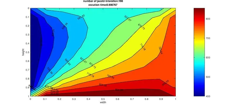
*Result of steady state analysis:-
i) Jacobi method:-
ii) Gauss seidel method:-
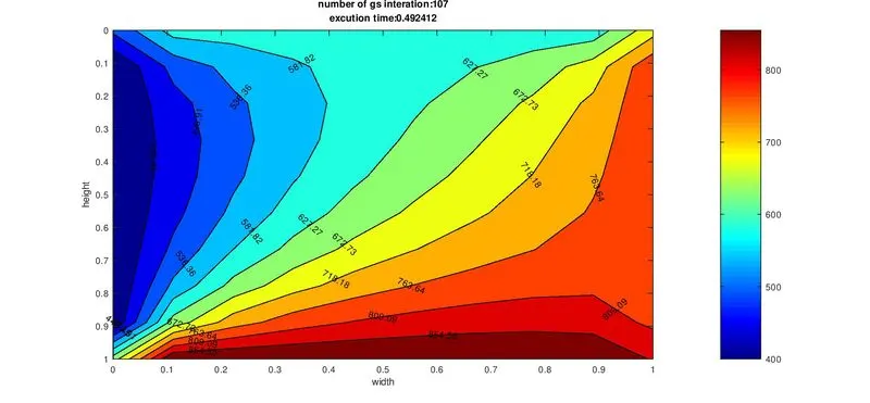
iii) SOR method:-
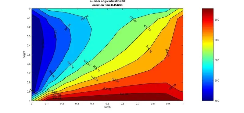
*Conclusion:-
-From this project we learn about 2D conduction heat transfer also learn temperature distribution in the 2D plate.
-For that we use numerical methods just like jacobi, gauss seidel and sor method.