Week 5.1 - Mid term project - Solving the steady and unsteady 2D heat conduction problem
Aim: To solve steady and unsteady two-dimensional heat conduction equations using implicit and explicit methods.
Objectives:
1. Write a MATLAB code to solve the steady-state two-dimensional heat conduction equation using the implicit method.
2. Write a MATLAB code to solve unsteady (transient) state two-dimensional heat conduction equation using the explicit method.
3. Write a MATLAB code to solve unsteady (transient) state two-dimensional heat conduction equation using the implicit method.
4. Plot the results and compare the efficacy of an iterative solver.
Theory:
The heat equation is the partial differential equation used to describe the distribution of some quantity (such as heat) over a domain from high concentration to low concentration as a function of time. Heat equation can be described in one, two, and three dimensions.
Three-dimensional heat conduction equation,
(delT)/(delt) +alpha*((del^2T)/(delx^2) +(del^2T)/(dely^2)+ (del^2T)/(delz^2)) = 0
Where,
(delT)/ (delt) = Rate of change of temperature as a function of time / Time derivative
(del^2T)/(delx^2) + (del^2T)/(dely^2) + (del^2T)/(delz^2) = Rate of change of temperature in cartesian co-ordinates (x,y,z) / Spatial derivatives
alpha = Thermal diffusivity of the medium.
However, in this analysis two-dimensional heat equation is used, it can be given as,
(delT)/(delt) +alpha*((del^2T)/(delx^2) +(del^2T)/(dely^2)) = 0
Types of methods:
1. Explicit method: In explicit methods, the parameters are calculated based on known values of previous time levels.
e.g: x^(n+1) = x^(n) + z^(n)
Here, LHS has the value to be evaluated and RHS has all the known values of the previous time-step.
2. Implicit method: In implicit methods, parameters are dependent on each other at the same time level.
e.g: x^(n+1) = x^(n) + z^(n+1)
Here, LHS has the value to be evaluated and RHS has the dependent value 'z^(n+1)' on 'x^n'. In simple words, both the LHS and RHS have unknown values (values to be calculated) which will be calculated as the iteration/generation progresses.
These methods are employed in solving steady and unsteady 2D heat conduction equations.
Derivation for steady and transient state two-dimensional heat conduction equation:
1. Steady-state two-dimensional heat conduction equation:
- Steady-state condition is independent of time.
- Steady state two dimensional heat conduction equation can be given as,
(del^2T)/(delx^2) +(del^2T)/(dely^2) = 0
- In laplacian, it can be written as,
triangle^2 T = 0
- In order to solve the above partial differential equation, we need to discretize the above equation using a second-order central difference approximation scheme.
- The heat equation is elliptic in nature. It can be inferred from `(del^2T)/(delx^2) +(del^2T)/(dely^2)`. For ellipse `(x^2)/(a^2) + (y^2)/(b^2)`.
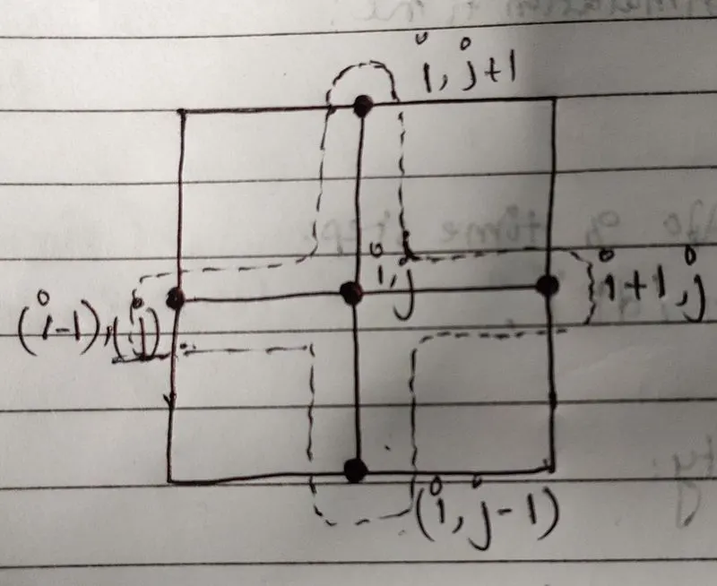
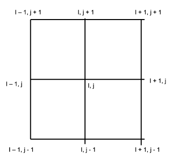
Here, a middle node is a concern for calculation and it will extract information from the left, right, bottom, and top nodes to evaluate itself.
(T_((i-1),j) - 2*T_(i,j) + T_((i+1),j))/(trianglex^2) + (T_(i,(j-1)) - 2*T_(i,j) + T_(i,(j+1)))/(triangley^2) = 0
Introducing some shortcuts for ease,
T_p = T(i,j)` ; `T_R = T_((i+1),j)` ; `T_L = T_((i-1),j)`; `T_T = T_(i,(j+1))` ; `T_B = T_(i,(j-1))
Now, simplifying the above equation, the equation becomes,
(T_(L) - 2*T_(p) + T_(R))/(trianglex^2) + (T_(B) - 2*T_(P) + T_(T))/(triangley^2) = 0
Assuming `trianglex^2 = triangley^2`, i.e. Equal discretization in X and Y dimensions (Nodes in X = Nodes in Y)
(T_(L) - 2*T_(p) + T_(R)+ T_(B) - 2*T_(P) + T_(T))/(trianglex^2) = 0
Upon further simplification, we get,
T_p = 1/4 * (T_L + T_R + T_B + T_T)
From the calculation point of view, the equation can be modified as,
T_(i,j) = 1/4 *(T_((i-1),j) + T_((i+1),j) + T_(i,(j-1)) + T_(i,(j+1)))
This is the final equation which will assist in calculating temperature distribution over a domain for steady state condition.
The steady-state heat conduction is solved by an implicit method using iterative solvers. The three types of iterative solvers are,
A) Jacobi Iteration Method
B) Gauss-Seidel Method
C) Successive Over-relaxation method
A) Jacobi Iteration Method:
In the Jacobi method, during the calculations for a particular iteration, the known values are all from the previous iteration.
2D steady state heat conduction equation can be given as,
T_(i,j)^(n+1) = 1/4 *(T_((i-1),j)^(n) + T_((i+1),j)^(n) + T_(i,(j-1))^(n) + T_(i,(j+1))^(n)
where,
T_(node position)^(n+1) denotes the new value to be calculated at time step 'n+1'
T_(node position)^(n)` denotes the calculated values at the previous/initial condition at time step 'n'
B) Gauss-Seidel Method:
In the Gauss-Seidel method, the resulted variables are used in further computations as soon as they are updated. The known values are a mix of variable values from the previous iteration as well as variable values that already have been updated in the current iteration.
2D steady state heat conduction equation for Gauss-Seidel method can be given as,
T_(i,j)^(n+1) = 1/4*(T_(i-1,j)^(n+1) + T_(i+1,j)^(n) + T_(i,j-1)^(n+1) + T_(i,j+1)^(n))
where,
T_(node position)^(n+1)` denotes the new value to be calculated at time step 'n+1'
T_(node position)^(n)` denotes the calculated values at the previous/initial condition at time step 'n'
C) Successive Over-relaxation method:
It is a variant of the Gauss-Seidel method for solving a linear system of equations, which results as a catalyst for convergence. It basically accelerates a slow iterative process and results in faster convergence.
It uses a relaxation factor that lies in between `0 < omega < 2`. Multiplying the relaxation factor to the original Gauss-Seidel equation and adding the difference of relaxation factor from unity and taking the product of the value resulted in the previous iteration enhances the speed of convergence.
2D steady state heat conduction equation for Successive Over-relaxation (SOR) method can be given as,
T_(i,j)^(n+1) = omega*(1/4*(T_(i-1,j)^(n+1) + T_(i+1,j)^(n) + T_(i,j-1)^(n+1) + T_(i,j+1)^(n)))+ (1-omega)*T_(i,j)^(n);
where,
omega` = Relaxation factor
T_(node position)^(n+1)` denotes the new value to be calculated at time step `n+1
T_(node position)^(n)` denotes the calculated values at the previous/initial condition at time step 'n'
2. Unsteady (Transient) state two-dimensional heat conduction equation:
The variation of temperature in time at any place within the domain is called Unsteady or Transient conduction. There is a time dependence of temperature fields in the domain.
Unsteady (Transient) state two-dimensional heat conduction equation can be given as,
(delT)/(delt) +alpha*((del^2T)/(delx^2) +(del^2T)/(dely^2)) = 0
In laplacian, it can be written as,
(delT)/(delt) +alphatriangle^2(T) = 0
Discretizing the partial differential equation by taking forward difference in time and central diffrence in space, we get,
`(T_(i,j)^(n+1) - T_(i,j)^(n))/(trianglet) + alpha*((T_((i-1),j) - 2*T_(i,j) + T_((i+1),j))/(trianglex^2))^(
Using similar shortcuts as above, the equation becomes,
`T_(P)^(n+1) = T_(P)^(n) + alphatrianglet((T_(L) - 2*T_(P) + T_(R))/(trianglex^2) + (T_(B) - 2*T_(P) + T_(T))/(triangley^2))^(n)`
The above equation is 2D transient heat conduction equation obtained by using explicit method.
And for Implicit method, recall the above equation, and change the time step to (n+1),
`T_(P)^(n+1) = T_(P)^(n) + alphatrianglet((T_(L) - 2*T_(P) + T_(R))/(trianglex^2) + (T_(B) - 2*T_(P) + T_(T))/(triangley^2))^(n+1)`
Introducing some constants,
`k1 = (alphatrianglet)/(trianglex^2)
Simplifying the above equation,
`T_(P)^(n+1) = T_(P)^(n) + k1 (T_(L)^(n+1) - 2T_(P)^(n+1) + T_(R)^(n+1)) + k2(T_(B)^(n+1) - 2T_(P)^(n+1) + T_(T)^(n+1))`
Taking all the (n+1) terms to the left side of the equation, we get,
`T_(P)^(n+1)- k1 *T_(L)^(n+1) + 2k1*T_(P)^(n+1) -k1* T_(R)^(n+1) - k2*T_(B)^(n+1) + 2k2*T_(P)^(n+1) - k2*T_(T)^(n+1) = T_(P)^(n)`
Taking `T_(P)^(n+1)` common, then equation becomes,
`T_(P)^(n+1) (1+2k1 + 2k2) - k1*T_(L)^(n+1) - k1*T_(R)^(n+1) -k2*T_(B)^(n+1) -k2*T_(T)^(n+1)= T_(P)^(n)`
Transferring `(1+2k1 + 2k2)` to the right side of the equation, we get,
`T_(P)^(n+1) = ((T_(P)^(n) + k1(T_(L)^(n+1) + T_(R)^(n+1)) + k2(T_(B)^(n+1) + T_(T)^(n+1)))/(1+2k1+2k2))`
Note: For any iteration,
T_(P)^(n)= This value will be known/input and it should not change within an iteration.
And, all the values except the above stated must change with/within each iteration.
From calculation point of view, the above equation can be modified as,
T_(i,j)^(n+1) = (T_(i,j)^(n) + k1(T_((i-1),j)^(n+1)+ T_((i+1),j)^(n+1)) + k2(T_(i,(j-1))^(n+1)+ T_(i,(j+1))^(n+1)))/(1+2k1+
This is 2D transient heat conduction equation obtained by using implicit method.
Implicit method:
To calculate Unsteady (Transient) state heat conduction by an implicit method using iterative solvers. The three types of iterative solvers are,
A) Jacobi Iteration Method
B) Gauss-Seidel Method
C) Successive Over-relaxation method
A) Jacobi Iteration Method:
The unsteady-state heat conduction equation using the Jacobi Iteration method can be given as,
T_(i,j)^(n+1) = (T_(i,j)^(n) + k1(T_((i-1),j)^(n)+ T_((i+1),j)^(n)) + k2(T_(i,(j-1))^(n)+ T_(i,(j+1))^(n)))/(1+2k1+2k2)
As in Jacobi's Iteration method, all the known values of temperature are taken from the previous iteration / initial condition and the new temperature is calculated accordingly.
B) Gauss-Seidel Method:
The unsteady-state heat conduction equation using the Gauss-Seidel method can be given as,
T_(i,j)^(n+1) = (T_(i,j)^(n) + k1(T_((i-1),j)^(n+1)+ T_((i+1),j)^(n)) + k2(T_(i,(j-1))^(n+1)+ T_(i,(j+1))^(n)))/(1+2k1+2k2)
Here in the Gauss-Seidel method, as soon as the previous values get updated, they are used in computation within an iteration.
C) Successive Over-relaxation method:
The unsteady-state heat conduction equation using the Successive Over-relaxation (SOR) method can be given as,
T_(i,j)^(n+1) = omega*((T_(i,j)^(n) + k1(T_((i-1),j)^(n+1)+ T_((i+1),j)^(n+1)) + k2(T_(i,(j-1))^(n+1)+ T_(i,(j+1))^(n+1)))/(1+2k1+
The SOR method generally modifies the gauss seidel a bit by introducing a constant called as relaxation factor. By using this method to a slow iterative process, the speed of convergence gets enhanced.
Here modifying `omega such that `omega>1`is termed as Over-relaxation and `omega<1`is known as Under-relaxation. By using the over-relaxation factor, the number of iterations required to meet convergence criteria gets reduced.
The above resulted from all the equations will assist to solve the steady and unsteady state 2D heat conduction equation.
INPUT PARAMETERS AND BOUNDARY CONDITIONS:
Assumptions:
The length of the domain = l = 1m;
Nodes in x and y dimensions = nx = ny = 10;
The initial temperature of the domain irrespective of the boundary condition = 300 K
Boundary conditions:
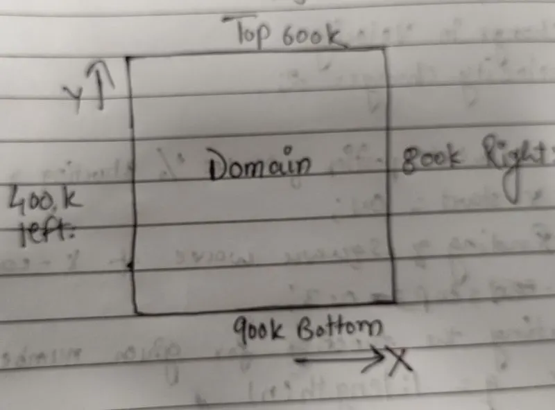
1. Steady-state two-dimensional heat conduction equation:
Implicit Method:
MATLAB code:
% CODE TO SOLVE TWO DIMENSIONAL HEAT CONDUCTION EQUATION
% Steady heat conduction equation is given as,
%(d^2T/dx^2 + d^2T/dy^2)= 0
%% Implicit method
clear all
close all
clc
% Length of the domain
l = 1;

% To discretize the domain
% X variables
nx = 10;
x = linspace(0,l,nx);
dx = l/(nx-1);

% Y variables
ny = 10;
y = x;
dy = l/(ny-1);

% Apply boundary condition to the domain
Tl = 400;
Tr = 800;
Tb = 900;
Tt = 600;

% Initializing temperature
T  = 300*ones(nx,ny);

% Temperature distribution at the boundaries
T(2:ny -1,1)= Tl;
T(2:ny -1,nx)= Tr;
T(1,2:nx - 1) = Tt;
T(ny,2:nx - 1) = Tb;

% Temperature at the corners
T(1,1) = (Tl+Tt)/2;
T(1,end) = (Tr+Tt)/2;
T(end,end) = (Tr+Tb)/2;
T(end,1) = (Tl+Tb)/2;

% Creating duplicate variables
T_initial = T;
T_old = T;

% Various inputs
error = 9e9;
acc = 1e-4;                  % Accuracy expected
jacobi_iter = 0;             % Initialize jacobi iteration method
gauss_seidel_iter = 0;       % Initialize gauss seidel iteration method
sor_iter = 0;                % Initialize succesive over-relaxation method method
omega = 1.3;                 % Relaxation factor

iterative_solver = input('Iterative_solver = ')

%% Jacobi's method
if iterative_solver ==1
  while  (error>acc)
       for i = 2:nx-1
           for j = 2:ny-1
              T(i,j) = 0.25*(T_old(i-1,j) + T_old(i+1,j) + T_old(i,j-1) + T_old(i,j+1));
           end
       end
       error = max(max(abs(T_old-T)));
           T_old = T;
           jacobi_iter = jacobi_iter+1;
  end
  figure(1)
contourf(x,fliplr(y),T,'ShowText','ON')
colorbar
colormap(jet)
title(sprintf('No. of Iterations (Jacobi method) = %d',jacobi_iter))
xlabel('X axis')
ylabel('Y axis')
end


%% Gauss-seidel method
if iterative_solver ==2
  while  (error>acc)
       for i = 2:nx-1
           for j = 2:ny-1
             T(i,j) = 0.25*(T(i-1,j) + T_old(i+1,j) + T(i,j-1) + T_old(i,j+1));
           end
       end
       error = max(max(abs(T_old-T)));
       T_old = T;
       gauss_seidel_iter = gauss_seidel_iter+1;
  end
figure(2)
contourf(x,fliplr(y),T,'ShowText','ON')
colorbar
colormap(jet)
title(sprintf('No. of Iterations (Gauss seidel method) = %d',gauss_seidel_iter))
xlabel('X axis')
ylabel('Y axis')
end


%% Successive over-relaxation method
if iterative_solver ==3
  while  (error>acc)
       for i = 2:nx-1
           for j = 2:ny-1
               T(i,j) = omega*(0.25*(T(i-1,j) + T_old(i+1,j) + T(i,j-1) + T_old(i,j+1)))+ (1-omega)*T_old(i,j);
           end
       end
       error = max(max(abs(T_old-T)));
       T_old = T;
       sor_iter = sor_iter+1;
  end
figure(3)
contourf(x,fliplr(y),T,'ShowText','on')
colorbar
colormap(jet)
title(sprintf('No. of Iterations (SOR method) = %d',sor_iter))
xlabel('X axis')
ylabel('Y axis')
end
Results:
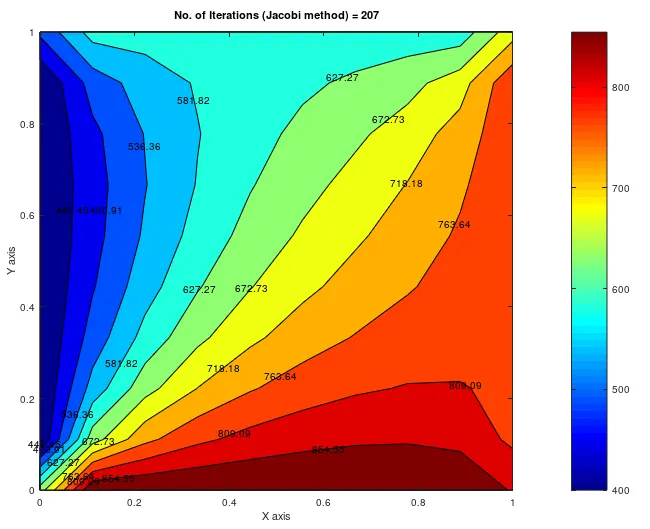
A) Jacobi Iteration method:
B) Gauss-Seidel method:
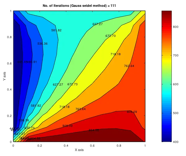
C) Successive Over-relaxation method:
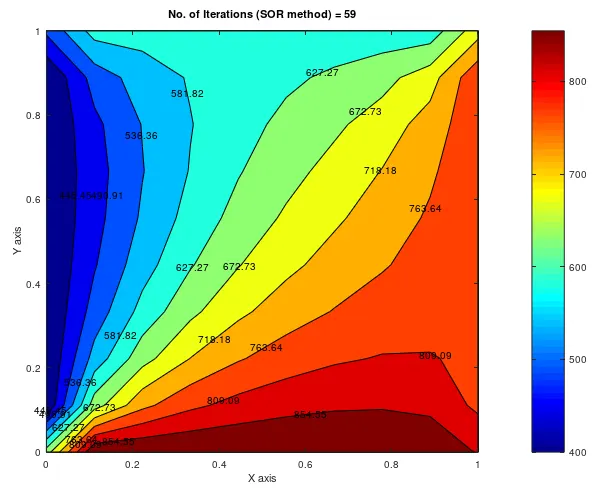
Explanation of the results obtained:
In the steady-state analysis, various implicit methods were applied to calculate the iterations required to achieve convergence. However, Jacobi's iterative solver took 207 iterations, Gauss-Seidel took 111 iterations and the SOR method resulted in convergence in just 59 iterations. This variation is due to the algorithm a particular iterative solver follows.
Additionally, the temperature distribution over the domain clearly shows the maximum diffusion (In heat conduction) at the bottom boundary as the temperature at the bottom boundary is the maximum. The flow of vibrational kinetic energy by the molecular movement from high temperature to low temperature can be visualized. The temperature distribution inside the domain is fairly simple that, respective to the boundary temperature, the flow of temperature results. It is nothing but the physical diffusion escalated over the domain obeying diffusion phenomena.
2. Unsteady (Transient) state two-dimensional heat conduction equation:
I] Explicit method:
MATLAB code:
% CODE TO SOLVE TWO DIMENSIONAL HEAT CONDUCTION EQUATION
% Transient heat conduction equation is given as,
%(dT/dt)+alpha*(d^2T/dx^2 + d^2T/dy^2) = 0
%% Explicit method
clear all
close all
clc
% Length of the domain
l = 1;

% To discretize the domain
% X variables
nx = 10;
x = linspace(0,l,nx);
dx = l/(nx-1);

% Y variables
ny = 10;
y = x;
dy = l/(ny-1);

% Time step
dt = 1e-3;

% Constants
alpha = 1.1;
k1 = (alpha*dt)/(dx^2);
k2 = (alpha*dt)/(dy^2);

% Apply boundary condition to the domain
Tl = 400;
Tr = 800;
Tb = 900;
Tt = 600;

% Initializing temperature
T  = 300*ones(nx,ny);

% Temperature distribution at the boundaries
T(2:ny -1,1)= Tl;
T(2:ny -1,nx)= Tr;
T(1,2:nx - 1) = Tt;
T(ny,2:nx - 1) = Tb;

% Temperature at the corners
T(1,1) = (Tl+Tt)/2;
T(1,end) = (Tr+Tt)/2;
T(end,end) = (Tr+Tb)/2;
T(end,1) = (Tl+Tb)/2;

% Creating duplicate variables
T_initial = T;
T_old = T;

% Various inputs
acc = 1e-4;   % Accuracy expected
conv = 9e9;  % Initialize convergence
error = 9e9;
explicit_iter = 0;

%% Explicit method

  while  (error>acc)
       for i = 2:nx-1
           for j = 2:ny-1
              term1 = T_old(i,j);
              term2 = k1*(T_old(i-1,j)- 2*T_old(i,j) + T_old(i+1,j));
              term3 = k2*(T_old(i,j-1)- 2*T_old(i,j) + T_old(i,j+1));
              T(i,j) = term1+term2+term3;
           end
       end
       error = max(max(abs(T_old-T)));
           T_old = T;
           explicit_iter = explicit_iter+1;
  end
figure(1)
contourf(x,fliplr(y),T,'ShowText','ON')
colorbar
colormap(jet)
title(sprintf('No. of Iterations (Explicit method) = %d',explicit_iter))
xlabel('X axis')
ylabel('Y axis')
Results:
Explicit method:
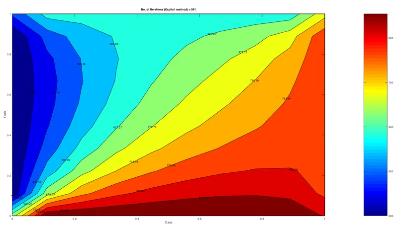
Explanation of the results obtained:
In a transient analysis by using an explicit method, 541 iterations are involved to converge a solution. As we know, explicit schemes are stable with smaller time-steps and do calculate the new value of a quantity based on the previous time-step. The temperature is displayed as above showing various temperatures at different nodes and elements as dependent on the boundary conditions.
II] Implicit method:
MATLAB Code:
% CODE TO SOLVE TWO DIMENSIONAL HEAT CONDUCTION EQUATION
% Transient heat conduction equation is given as,
%(dT/dt)+alpha*(d^2T/dx^2 + d^2T/dy^2) = 0
%% Implicit method
clear all
close all
clc
% Length of the domain
l = 1;

% To discretize the domain
% X variables
nx = 10;
x = linspace(0,l,nx);
dx = l/(nx-1);

% Y variables
ny = 10;
y = x;
dy = l/(ny-1);

% Time step
dt = 1e-3;

% Constants
alpha = 1.1;
k1 = (alpha*dt)/(dx^2);
k2 = (alpha*dt)/(dy^2);

% Apply boundary condition to the domain
Tl = 400;
Tr = 800;
Tb = 900;
Tt = 600;

% Initializing temperature
T  = 300*ones(nx,ny);

% Temperature distribution at the boundaries
T(2:ny -1,1)= Tl;
T(2:ny -1,nx)= Tr;
T(1,2:nx - 1) = Tt;
T(ny,2:nx - 1) = Tb;

% Temperature at the corners
T(1,1) = (Tl+Tt)/2;
T(1,end) = (Tr+Tt)/2;
T(end,end) = (Tr+Tb)/2;
T(end,1) = (Tl+Tb)/2;

% Creating duplicate variables
T_initial = T;
T_old = T;
T_prev = T;
T_x = T;

% Various inputs
acc = 1e-4;   % Accuracy expected
jacobi_iter = 0; % Initialize jacobi iteration method
gauss_seidel_iter = 0; % Initialize gauss seidel iteration method
sor_iter = 0; % Initialize successive over-relaxation method
t_iter = 0; % Initialize time iteration

conv = 9e9;  % Initialize convergence
omega = 1.1;  % Relaxation factor

% Prompt for calling methods.
iterative_solver = input('Iterative solver = ')

%% Jacobi's method
if iterative_solver ==1
 while  (conv>acc)
     error = 9e9;  % Initialize error
  while  (error>acc)
       for i = 2:nx-1
           for j = 2:ny-1
              term1 = 1/(1+(2*k1)+(2*k2));
              term2 = k1*term1;
              term3 = k2*term1;
              H = (T_old(i-1,j) + T_old(i+1,j));
              V = (T_old(i,j-1) + T_old(i,j+1));

              T(i,j) = (T_prev(i,j)*term1) + (H*term2) + (V*term3);
           end
       end
       error = max(max(abs(T_old-T)));
           T_old = T;
           jacobi_iter = jacobi_iter+1;
  end
           t_iter = t_iter + 1;
           conv = max(max(abs(T_prev-T)));
           T_prev = T;
 end
  figure(1)
contourf(x,fliplr(y),T,'ShowText','ON')
colorbar
colormap(jet)
title(sprintf('No. of Iterations (Jacobi method) = %d',jacobi_iter))
xlabel('X axis')
ylabel('Y axis')
end

%% Gauss-seidel method
if iterative_solver ==2
 while  (conv>acc)
     error = 9e9;  % Initialize error
  while  (error>acc)
       for i = 2:nx-1
           for j = 2:ny-1
              term1 = 1/(1+(2*k1)+(2*k2));
              term2 = k1*term1;
              term3 = k2*term1;
              H = (T(i-1,j) + T_old(i+1,j));
              V = (T(i,j-1) + T_old(i,j+1));

              T(i,j) = (T_prev(i,j)*term1) + (H*term2) + (V*term3);
           end
       end
       error = max(max(abs(T_old-T)));
           T_old = T;
           gauss_seidel_iter = gauss_seidel_iter+1;
  end
           t_iter = t_iter + 1;
           conv = max(max(abs(T_prev-T)));
           T_prev = T;
 end
 figure(2)
contourf(x,fliplr(y),T,'ShowText','ON')
colorbar
colormap(jet)
title(sprintf('No. of Iterations (Gauss seidel method) = %d',gauss_seidel_iter))
xlabel('X axis')
ylabel('Y axis')
end


%% Successive over-relaxation method
if iterative_solver ==3
 while  (conv>acc)
     error = 9e9;  % Initialize error
  while  (error>acc)
       for i = 2:nx-1
           for j = 2:ny-1
              term1 = 1/(1+(2*k1)+(2*k2));
              term2 = k1*term1;
              term3 = k2*term1;
              H = (T(i-1,j) + T_old(i+1,j));
              V = (T(i,j-1) + T_old(i,j+1));

              T(i,j) = (T_prev(i,j)*term1) + (H*term2) + (V*term3);
              T_x(i,j) = ((1-omega)*T_old(i,j))+ (T(i,j)*omega);
           end
       end
       error = max(max(abs(T_old-T)));
           T_old = T_x;
           sor_iter = sor_iter+1;
  end
           t_iter = t_iter + 1;
           conv = max(max(abs(T_prev-T)));
           T_prev = T;
 end
figure(3)
contourf(x,fliplr(y),T,'ShowText','ON')
colorbar
colormap(jet)
title(sprintf('No. of Iterations (SOR method) = %d',sor_iter))
xlabel('X axis')
ylabel('Y axis')
end
Results:
Implicit method:
1. Jacobi Iteration Method:
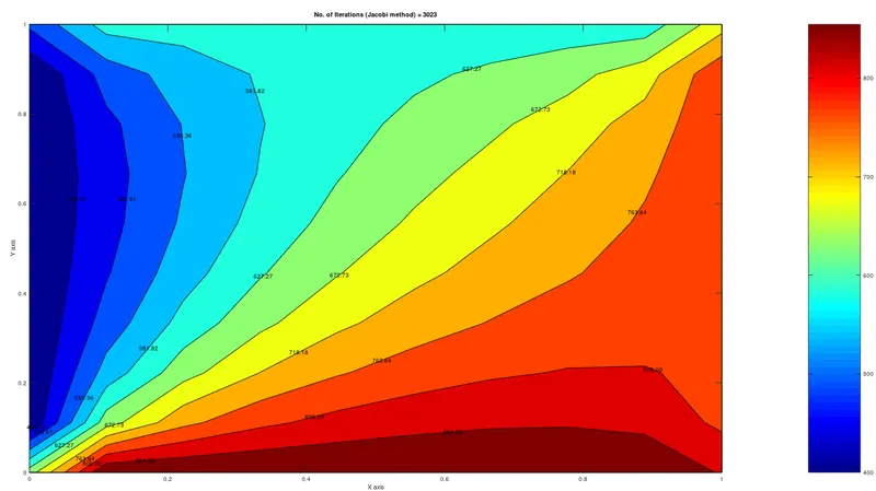
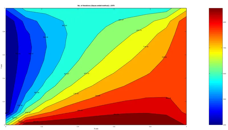
2. Gauss-Seidel Method:
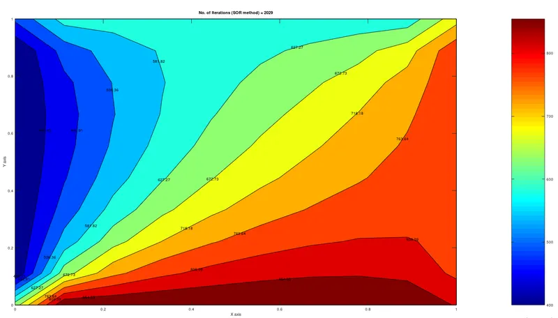
3. Successive Over-relaxation Method:
Explanation of the results:
Temperature distribution graphs are calculated using Implicit methods. The temperature at the new time-step is being evaluated using the information from the previous time-step as well as from the ongoing time-step resulting in a set of simultaneous equations. Here, Jacobi's iterative method took 3023 iterations, Gauss-Seidel took 2470 iterations and the SOR method took 2029 iterations to converge a solution to expected accuracy. This is because the over-relaxation factor speeds up the iterative algorithm. Here over-relaxation factor ('omega = 1.1') gives optimal results, varying it above or below increases the iterative behavior of the method. However, different iterative solvers obey different algorithms to converge a solution because of that variation of iterations, and time dependency comes into the picture giving similar results at various computation times and iterations. The temperature distribution is spread over the domain because of the temperature gradient along the boundary of a domain.
Observation Table:
| Type of two-dimensional heat conduction state | No.of iterations using Explicit method |
No.of iterations using Jacobi iterative method (Implicit Method) |
No.of iterations using Gauss-Seidel method (Implicit Method) |
No.of iterations using Successive Over-relaxation method (Implicit Method) |
| Steady State | NA | 207 | 111 | 59 |
| Unsteady (Transient) state | 541 | 3023 | 2470 | 2029 |
Key result:
In terms of iterations, Jacobi Iteration method > Gauss-Seidel method > Successive Over-relaxation method.
In terms of convergence speed, Jacobi Iteration method < Gauss-Seidel method < Successive Over-relaxation method.
Summary:
In this project, a two-dimensional heat conduction equation is solved for steady and unsteady state conditions using the explicit and implicit methods. Initially, steady-state was solved using Implicit methods with the use of different iterative solvers (Jacobi, Gauss-Seidel, and SOR). Each iterative solver calculated steady-state with certain iterations and computation time. In which the SOR method shown effective results as compared to Jacobi and Gauss-Seidel. As the number of iterations involved in the SOR method was comparatively less and faster convergence was achieved. Similarly, in transient analysis using the explicit method, the transient behavior of temperature was reached to steady-state over a period of time (`T_(i,j)^(n+1) = T_(i,j)^(n)`) or in other words, the convergence of the solution was achieved to a defined accuracy. The transient analysis using the implicit method resulted in various iterations for the convergence of the solution. Again for a particular iterative solver, iterating time, computation time and speed of convergence differ respectively. Also, in transient analysis, the SOR method shown lean and effective iteration steps and a faster speed of convergence as compared to other iterative solvers.
Conclusion:
The application of an iterative solver for numerical computing either results in convergence or divergence of the solution. While considering the case of convergence, the significant matter of concern in CFD analysis is the speed of convergence of the solution and required computation time. Different iterative solvers possess different algorithms with which numerical problems are solved. Again there is a need for adopting the implicit and explicit methods for a given problem. It certainly depends upon the given conditions and results to be expected. In this project, explicit schemes tend to be more effective as compared to implicit schemes for transient analysis, however, it was only possible because the time-step involved was very less and therefore the stable solution has resulted. But, if time step conditions vary, one cannot rely on an explicit scheme to get stable results. As they tend to be unstable for larger time-step and smaller element discretization. So implicit schemes are usually preferred for their stability and for larger time-steps variation.