Week 3 - Solving second order ODEs

Aim - To solve the second-order ODE function for a pendulum by using Matlab and simulate the motion.

Theory for pendulum

A pendulum is a mass attached with a string suspended from a pivot so that it can swing freely. It is subjected to a restoring force which accelerated it back to normal in an equilibrium position, the movement of back and forth of motion of a pendulum is known as a period. The pendulum oscillates freely from its suspension. The motion that we see in the pendulum is totally dependent on the length of the string and the initial angular displacement provided.

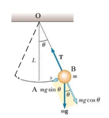
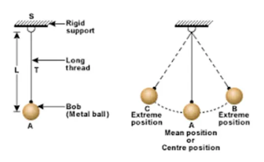
Fig(a) nomenclature of pendulum fig(b) swing positions

The real pendulum works on the principle of 'NEWTONS SECOND LAW OF MOTION', where the pendulum is subjected to friction and air drag which reduces the amplitude and motion of string cycle by cycle. According to newtons second law, it states that "the rate of change of the momentum of the body with time is directly proportional to the force applied and bring back to the position where the force is applied on it i.e in the direction from where the force is applied, this is why the body produces a proportional acceleration.

F = m*a

where,

F= force (N)

m= mass

a= acceleration

Objective -

(a) Write a program to solve the ODE which represents the equation of motion of a simple pendulum with damping.

following is the ODE about a simple pendulum.

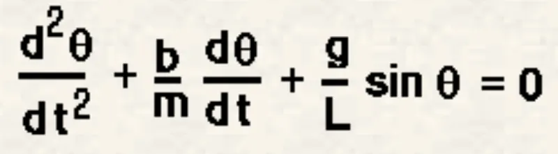
where,

g = gravity in m/s^2,

L = length of the pendulum in m,

m = mass of the ball in kg,

b= damping coefficient.

(B) simulate the motion of pendulum body

Here, To solve the ODE, we assign the value of the input which are given to the pendulum.

L=1 metre,

m=1 kg,

b=0.05.

g=9.81 m/s^2.

time period(t_span) = 0-20 sec

angular displacement=0

angular velocity=3 rad/sec at time t=0.

Procedures

To calculate the second-order oDE, we need to break it into first order for coding and calculation purposes and then form a solution matrix for results.

MATLAB CODE

%breaking second order ode and form solution matrix

%Defining function

function [dtheta_dt] = pend_func(t,theta,b,g,l,m);
theta1 = theta(1);
theta2 = theta(2);
dtheta1_dt = theta(2);
dtheta2_dt = (-b/m)*theta2-(g/l)*sin(theta1);
dtheta_dt = [dtheta1_dt;dtheta2_dt];
end

In this function, the simplified second order ode by simplifying theta1 and theta2. the respective value of theta1 and theta2 are assigned and differentiated it and putting all the values together in the solution matrix.

2) created the main function script and specify all the values or parameters, the initial time span and condition is defined. The inbuilt Matlab solver named 'ode45' is used to solve the function. This function implements the Runge-Kutta method with a variable time step for efficient computation with minimum error propagation.

clear all
close all
clc

%input conditions 
b = 0.05;
g = 9.81;
l = 1;
m = 1;

% initial conditions 

theta_0 = [0;3];

%time point
t_span = linspace(0,20,300);
%solve ode
[t,results] = ode45(@(t,theta) pend_func(t,theta,b,g,l,m),t_span,theta_0);

Here, in this main function, we used 'linspace' command for time span in order to get results at a various time step, finally, the calculated results are as follow.

Results

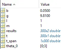
3) in this step we will be plotting and labeling the following outcome.

MATLAB CODE

%plotting figure(1)
title('Relationship Between Angular Displacement And Angular Velocity w.r.t. Time')
hold on
plot(t,results(:,1))
plot(t,results(:,2))
grid on
xlabel('time(sec)')
legend('Angular Displacement(rad)','Angular Velocity(rad/sec)')

Results

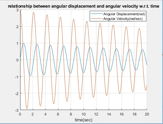
observing the above result we can conclude is that the angular displacement w.r.t angular velocity is changing, certainly, both are decreasing w.r.t time as inclusion of damping at pivot point

% to plot and animate pendulum
ct=1
for i = 1:length(results(:,1));

% co-ordinates
x0 = 0
y0 = 0
x1 = l*sin(results(i,1));
y1 = -l*cos(results(i,1));

figure (2)
plot([-1 1],[0 0],'linewidth',3,'color','r')
axis([-3 3 -3 3])
hold on
plot([x0 x1],[y0 y1],'linewidth',3,'color','g')
plot([x0 x1],[y0 y1],'o','Markersize',15,'MarkerFaceColor','r','MarkerEdgeColor','r')
grid on
pause (0.01)
M(ct) = getframe(gcf)
hold off
ct = ct+1;
end
%movie commands
movie(M)
video_file = VideoWriter('pendulum_challenge.avi','uncompressed AVI')
open(video_file)
writeVideo(video_file,M)
close(video_file)

result

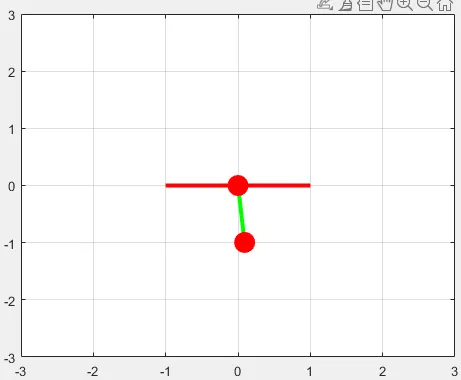
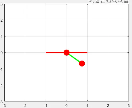
Animation

The following will be the youtube link of animation of a simple pendulum.

https://www.youtube.com/watch?v=6WwDRyvP0-c

error occurred

hold on retains the current plot and certain axes properties so that subsequent graphing commands add to the existing graph.

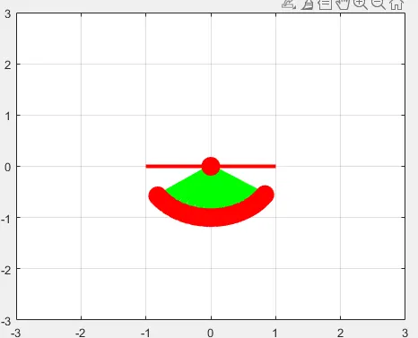
to overcome this problem I use the hold-off command because sets axis properties to their defaults before drawing new plots. and after using the hold-off command the error that occurred is corrected.