Aim: To derive a 4th order approximation of a 2nd order derivative using the Taylor table method.

Objectives:

1. Derive 4th order approximation of a second-order derivative using central, skewed right side, and skewed left side difference approximation method.

2. Prove that the approximation schemes are of fourth-order.

3. Write a program in MATLAB that evaluates a second-order derivative of an analytical function and compares results with these three numerical approximation schemes.

PART A: Derivation

1] Central difference method:

To compute the central difference method of fourth-order for a second-order derivative, we must follow the formula for calculating the number of node points.

'n = A + O - 1'

where,

n = Number of nodes in stencil

A = Accuracy of the approximation method

O = Order of the numerical function

Here, in our case A = 4; O = 2

So , n = 4+2 -1= 5

We have 5 number of node points for this approximation technique. Similarly, in central difference method with 5 number of nodes, two points will be placed on the left and two points will be placed on the right side of the node point i.e. (x)

The position of these four node points are `f(x-2dx),f(x-dx),f(x+dx),f(x+2dx)`. Here "`dx`" is the step node size.

The fourth order central difference approximation method is given by,

`(d^2f)/(dx^2) = af(x-2dx)+bf(x-dx)+cf(x)+d(x+dx)+ef(x+2dx) rightarrow A`

The values of co-efficients a,b,c,d and e are computed with the help of Taylor's table,

	`f(x)`	`f'(x)dx`	`f''(x)dx^2`	`f'''(x)dx^3`	`f''''(x)dx^4`	`f^(v)(x)dx^5`	`f^(vi)(x)dx^6`
`af(x-2dx)`	a	-2a	2a	-8a/6	2a/3	-4a/15	4a/45
`bf(x-dx)`	b	-b/2	b/2	-b/6	b/24	-b/120	b/720
`cf(x)`	c	0	0	0	0	0	0
`df(x+dx)`	d	d/2	d/2	d/6	d/24	d/120	d/720
`ef(x+2dx)`	e	2e	2e	8e/6	2e/3	4e/15	4e/45
`sum_(columns)`	0	0	1	0	0	?	?

Using the above Taylor table, we can write the equations of fourth order central approximation in the form of equation,

`a+b+c+d+e+h = 0 rightarrow 1`

`-2a-b+0+d+2e = 0 rightarrow 2`

`dx^2(2a + b/2 + 0 +d/2 + (2e))/(2) = 1`

Here, lets ignore `dx^2` for now, we will call it later,

Then the equation becomes,

`2a + b/2 + 0 +d/2 + 2e = 1 rightarrow 3`

`-(8a)/6-b/6+0+d/6+(8e)/6 = 0 rightarrow 4`

`(2a)/3 + b/24 + 0 + d/24 + (2e)/3 = 0 rightarrow 5`

Note: We can ignore the 6th equation as of now, as we are interested in calculating 5 unknowns and we need 5 equations for that. The 6th equation will be associated with `f^(vi)(x)dx^6`.

Now, writing those equations in the form of matrix in MATLAB,

AX = B

Then by matrix multiplication, the resulted coefficients are,

a = -0.0833; b = 1.3333; c = -2.5000; d = 1.3333; e = -0.0833

Here, we can see that a = e and b = d and substitute those values in equation A,

And the fourth order central difference approximation for the second derivative can be obtained as,

`(d^2f)/(dx^2) = (-0.0833f(x-2dx) + 1.3333f(x-dx) - 2.5f(x) + 1.3333f(x+dx) -0.0833f(x+2dx))/(dx^2)`

Proof of fourth order approximation scheme:

Expand Taylor table with only higher order terms,

`(d^2f)/(dx^2) = [f''(x) dx^2(2a + b/2+0+d/2+2e) + f^v(x)dx^5((-4a)/15-b/120+0+d/120+(4e)/15) +f^(vi)(x)dx^6((-4a)/45+b/720+0+d/720+(4e)/45)]`

Then the terms associated with `f^(v)(x)dx^5`gets cancelled, as a = e and b = d, so they cancel out each other.

`(d^2f)/(dx^2) = [f''(x) dx^2(2a + b/2+0+d/2+2e) +f^(vi)(x)dx^6((-4a)/45+b/720+0+d/720+(4e)/45)]`

Substituting the initial correlation, with '(d^2f)/(dx^2)'

af(x-2dx)+bf(x-dx)+cf(x)+d(x+dx)+ef(x+2dx) = [f''(x) dx^2(2a + b/2+0+d/2+2e) +f^(vi)(x)dx^6((-4a)/45+b/720+0+d/720+(4e)/45)]

dividing the above equation by 'dx^2'

(af(x-2dx)+bf(x-dx)+cf(x)+d(x+dx)+ef(x+2dx))/(dx^2) = [f''(x) (2a + b/2+0+d/2+2e) +f^(vi)(x)dx^4((-4a)/45+b/720+0+d/720+(4e)/45)]

In the right hand side of the equation, the first dx term has power 4, hence by ignoring this term with associated higher order terms, we get,

(af(x-2dx)+bf(x-dx)+cf(x)+d(x+dx)+ef(x+2dx))/(dx^2) = [f''(x) (2a + b/2+0+d/2+2e) +(0)f^(vi)(x)dx^4]

As neglecting the first higher order term with dx of power 4 implies that the truncation error is associated with the function is of order 4. Hence it is known to be as "Fourth order approximation scheme".

2] Skewed Right-sided method:

In the fourth-order right side skewed method, to calculate the fourth-order approximation of a second-order derivative of the function, we need to estimate the number of node points for the calculations.

So for a skewed scheme, the number of node points are,

n = A+O

n = 4+2

n = 6

Here six (6) number of points are required to calculate the fourth order skewed right side approximation. The position of these 6 nodes can be given as `f(x), f(x+1), f(x+2), f(x+3), f(x+4), f(x+5)`.

The fourth order skewed right side approximation of a second derivative is given by,

`(d^2f)/(dx^2) = af(x) + bf(x+dx) + cf(x+2dx) + df(x+3dx) + ef(x+4dx) + hf(x+5dx) rightarrow B`

The values of the co-efficients a,b,c,d,e and h can be calculated by using Taylor table,

	`f(x)`	`f'(x)dx`	`f''(x)dx^2`	`f'''(x)dx^3`	`f''''(x)dx^4`	`f^(v)(x)dx^5`	`f^(vi)(x)dx^6`
`af(x)`	a	0	0	0	0	0	0
`bf(x+1)`	b	b	b	b	b	b	b
`cf(x+2)`	c	2c	4c	8c	16c	32c	64c
`df(x+3)`	d	3d	9d	27d	81d	243d	729d
`ef(x+4)`	e	4e	16e	64e	256e	1024e	4096e
`hf(x+5)`	h	5h	25h	125h	625h	3125h	15625h
`sum_(columns)`	0	0	1	0	0	0	?

Referring the above Taylor table, we can write equations for fourth order right side skewed approximation, we get,

a+b+c+d+e+h = 0 rightarrow 1

0 + b + 2c + 3d + 4e + 5h = 0 rightarrow 2

dx^2(0+b+4c + 9d + 16e + 25h)/2 = 1

Ignoring the 'dx^2' term, we will call it later, the equation becomes,

0+b+4c + 9d + 16e + 25h = 2 rightarrow 3

0 + b + 8c + 27d + 64e + 125h = 0 rightarrow 4

0 + b + 16c + 81d + 256e + 625h = 0 rightarrow 5

0 + b + 32c + 243d + 1024e + 3125h = 0 rightarrow 6

Note: We can ignore 7th equation as of now, as we are intrested in calculating 6 unknowns and we need 6 equations for that.

Now, writing those equations in matrix form as,

AX = B

Then by matrix multiplication, the co-efficients are,

a = 3.75; b = -12.8333; c = 17.8333; d = -13; e = 5.0833; h = -0.0833

Substituting the values of co-efficients in Equation B and the fourth order right side skewed difference approximation for the second derivative can be obtained as,

`(d^2f)/(dx^2) = (3.75f(x) -12.8333f(x+dx) + 17.8333f(x+2dx) - 13f(x+3dx) + 5.0833f(x+4dx) - 0.0833f(x+5dx))/(dx^2)`

Proof of fourth order approximation scheme:

Expand Taylor table with higher order terms,

`(d^2f)/(dx^2) = f''(x) dx^2(0 + b+4c+9d+16e+25h) + f^(vi)(x)dx^6(0+b+64c+729d+4096e+15625h) + ....`

Substituting initial correlation of `(d^2f)/(dx^2)`

`af(x) + bf(x+dx) + cf(x+2dx) + df(x+3dx) + ef(x+4dx) + hf(x+5dx) = f''(x) dx^2(0 + b+4c+9d+16e+25h) + f^(vi)(x)dx^6(0+b+64c+729d+4096e+15625h) + ....`

Now, dividing the equation by `dx^2`

`(af(x) + bf(x+dx) + cf(x+2dx) + df(x+3dx) + ef(x+4dx) + hf(x+5dx))/(dx^2) = f''(x)(0 + b+4c+9d+16e+25h) + f^(vi)(x)dx^4(0+b+64c+729d+4096e+15625h) + ....`

Neglecting the terms with higher order, we get,

`(af(x) + bf(x+dx) + cf(x+2dx) + df(x+3dx) + ef(x+4dx) + hf(x+5dx))/(dx^2) = f''(x)(0 + b+4c+9d+16e+25h) + (0) f^(vi)(x)dx^4`

Here, the first term associated with 'dx' has power of 4, which means after neglecting it, a truncation error related to the function will get involved, which will be of order 4.

3] Skewed Left-sided method:

To compute the left side skewed difference method of fourth-order for a second-order derivative, we must follow the formula for calculating the number of node points.

For a skewed scheme, the number of node points are,

n = A+O

n = 4+2

n = 6

Here six (6) number of points are required to calculate the fourth order left side skewed approximation. The position of these 6 nodes can be given as 'f(x-5dx), f(x-4dx), f(x-3dx), f(x-2dx), f(x-dx), f(x)'.

The fourth order skewed left side approximation of a second derivative is given by,

(d^2f)/(dx^2) = af(x-5) + bf(x-4) + cf(x-3) + df(x-2) + ef(x-1) + h(x)

The values of the co-efficients a,b,c,d,e and h can be calculated by using Taylor table,

	f(x)	f'(x)dx	f''(x)dx^2	f'''(x)dx^3	f''''(x)dx^4	f^(v)(x)dx^5	f^(vi)(x)dx^6
'af(x-5)'	a	-5a	25a	-125a	625a	-3125a	15625a
'bf(x-4)'	b	-4b	16b	-64b	256b	-1024b	4096b
'cf(x-3)'	c	-3c	9c	-27c	81c	-243c	729c
'df(x-2)'	d	-2d	4d	-8d	16d	-32d	64d
'ef(x-1)'	e	-e	e	-e	e	-e	e
'h(x)'	h	0	0	0	0	0	0
'sum_(columns)'	0	0	1	0	0	0	?

By observing the above Taylor table, we can write equations for fourth order left side skewed approximation,

a + b + c + d + e + h = 0 rightarrow 1

-5a - 4b -3c -2d - e - 0 = 0 rightarrow 2

dx^2(25a + 16b + 9c + 4d + e + 0)/2 = 1

Here, let's again neglect `dx^2`, we get the equation as,

25a + 16b + 9c + 4d + e + 0 = 2 rightarrow 3

-125a - 64b -27c -8d -e - 0 = 0 rightarrow 4

625a + 256b + 81c + 16d + e + 0 = 0 rightarrow 5

-3125a - 1024b - 243c - 32d - e - 0 = 0 rightarrow 6

Note: In the 7th equation, as we have 6 unknowns and we need 6 equations to calculate it.

Now, we will write those equations in the matrix form,

AX = B

Then by matrix multiplication, the coefficients are,

a = -0.8333; b = 5.0833; c = -13; d = 17.8333; e = -12.8333; h = 3.75

Substituting these values in Equation B and the fourth order skewed left side difference approximation for a second order derivative can be obtained as,

(d^2f)/(dx^2) = (-0.8333f(x-5dx) +5.0833f(x-4dx) -13 f(x-3dx) + 17.8333f(x-2dx) -12.8333f(x-dx) +3.75f(x))/(dx^2)

By observation, the coefficients of a skewed left-sided scheme are the same as a skewed right-sided scheme but in reverse order. It is obvious because both the approximation techniques are of the same accuracy and they both take information from 5 points to compute the value of the function. Conclusively, the proof provided for skewed right-sided approximation will satisfy the condition for skewed left-sided approximation. So no proof is provided separately for the skewed left-sided approximation method.

PART B: Evaluate a function using MATLAB

Analytical function is,

f(x) = exp(x)*cos(x)

and let's take `x = pi/3 and dx = (pi/3,pi/3000)`

MATLAB code:

Explanation:

In this OCTAVE programming, a second-order analytical function is evaluated by using fourth-order numerical approximation techniques.

• Initially, create the function file separately for different approximation techniques.
• In the function file, assign the input variables of the respective approximation schemes. Additionally, write the respective matrix for the particular scheme in order to find coefficients of the resulting approximation equations.

Note: Do not insert coefficients manually because the input parameters with limited recurring digits will create an additional error to the solution. So it is a better practice to insert coefficients in the form of fractions or instructing MATLAB to extract values from the given approximation matrix.

• Insert formula of the respective approximation scheme individually in different schemes and as an output to calculate the fourth-order error incurred in that dedicated approximation scheme.
• Create a new ".m file" which will have the main program.
• Start with clear all; close all; clc;
• Then define the input parameters like the value of "x", "range of dx" using linspace command, and "second-order derivative of the analytical function.
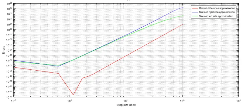
• Create a for loop to calculate the error along with dx, 200 being the number of intervals across the range of "dx'. Errors pertaining to the central, skewed right side, and skewed left side approximation schemes will be calculated inside the loop resulting in an array of 200 steps along with the "dx".
• After calculating the errors, plot them using the "log-log" command as it gives results in the logarithmic 10 base scale, which will facilitate interpreting results.
• Finally, insert the title, legend, and labels to display results in an effective manner.

Function file for central difference method

function err_central = central_diff(analytical_derivative,x,dx)
C = [1,1,1,1,1;-2,-1,0,1,2;2,1/2,0,1/2,2;-8/6,-1/6,0,1/6,8/6;2/3,1/24,0,1/24,2/3];
H = [0;0;1;0;0];
M = C\H;
% Central difference can be calculated as,
fourth_central = (M(1)*exp(x-2*dx)*cos(x-2*dx) + M(2)*exp(x-dx)*cos(x-dx) + M(3)*exp(x)*cos(x) + M(4)*exp(x+dx)*cos(x+dx) + M(5)*exp(x+2*dx)*cos(x+2*dx))./(dx^2);
err_central = abs(analytical_derivative - fourth_central)
end

2. Function code of skewed right side method

function err_right = right_side(analytical_derivative,x,dx)
R = [1,1,1,1,1,1;0,1,2,3,4,5;0,1,4,9,16,25;0,1,8,27,64,125;0,1,16,81,256,625;0,1,32,243,1024,3125]
H = [0;0;2;0;0;0];
N = R\H;
% Skewed right side difference can be calculated as,
fourth_right = (N(1)*exp(x)*cos(x) + N(2)*exp(x+dx)*cos(x+dx) + N(3)*exp(x+2*dx)*cos(x+2*dx) + N(4)*exp(x+3*dx)*cos(x+3*dx) + N(5)*exp(x+4*dx)*cos(x+4*dx) + N(6)*exp(x+5*dx)*cos(x+5*dx))./(dx.^2);
err_right = abs(analytical_derivative - fourth_right);
end

3. Function code of skewed left side method

function err_left = left_side(analytical_derivative,x,dx)
L = [1,1,1,1,1,1;-5,-4,-3,-2,-1,0;25,16,9,4,1,0;-125,-64,-27,-8,-1,0;625,256,81,16,1,0;-3125,-1024,-243,-32,-1,0];
H = [0;0;2;0;0;0];
O = L\H;
% Skewed left side difference can be calculated as,
fourth_left = (O(1)*exp(x-5*dx)*cos(x-5*dx) + O(2)*exp(x-4*dx)*cos(x-4*dx) + O(3)*exp(x-3*dx)*cos(x-3*dx) + O(4)*exp(x-2*dx)*cos(x-2*dx) + O(5)*exp(x-dx)*cos(x-dx) + O(6)*exp(x)*cos(x))./(dx.^2);
err_left = abs(analytical_derivative - fourth_left);
end

Main code:

clear all
close all
clc
% Inputs 
x = 2*pi
dx = linspace(pi/3,pi/3000,200);
% Analytical function f(x) = exp(x)*cos(x)
analytical_derivative = -2*exp(x)*sin(x);   % Second order analytical derivative
% Error of numerical derivative
for i=1:length(dx)
err_central(i) = central_diff(analytical_derivative,x,dx(i))
err_right(i) = right_side(analytical_derivative,x,dx(i))
err_left(i) = left_side(analytical_derivative,x,dx(i))  
end
% Plotting
loglog(dx,err_central,'r',dx,err_right,'b',dx,err_left,'g')
xlabel('Step size of dx')
ylabel('Errors')
grid on
legend('Central difference approximation','Skewed right side approximation','Skewed left side approximation')
title('Fourth order approximation') 

Result:

Significance of skewed scheme:

The central difference approximation scheme takes information from both the sides of the node point which to be evaluated i.e. in a symmetric manner. However, skewed schemes extract information from either side of the nodal position (It can be left or right). When the function or a nodal point is to be evaluated in space or domain, where it might have nodal points only in one direction i.e. either in right or left. In such instances, skewed schemes are preferred over central approximation schemes. Though the central difference approximation scheme is more significant in terms of accuracy still it loses its stance when it comes to calculating a function at the boundary of a domain.

Conclusion:

The displayed results show that the fourth-order central difference approximation method has the least error as compared to both fourth-order skewed schemes. The fourth-order central difference approximation method is effective because it takes the information from neighboring symmetrical nodes, which helps to approximate results precisely as compared to the skewed right and left side approximation schemes. However, sometimes for a wider range of step size, higher-order approximation techniques stood out to be inefficient as the error at any point is the net sum of a numerical error and round-off error. Higher-order approximation techniques have a high value of round-off error, so in such instances, lower-order approximation techniques are preferred for the accuracy of the solution.

Note: Random sampling of skewed distributions does not necessarily imply Taylor's law (Reference 4)

References:

1. https://www.statisticshowto.com/probability-and-statistics/skewed-distribution/

2. https://www.pnas.org/content/112/25/7749

3. https://core.ac.uk/download/pdf/214328356.pdf

4. https://www.ncbi.nlm.nih.gov/pmc/articles/PMC4485107/