Week 5.1 - Mid term project - Solving the steady and unsteady 2D heat conduction problem
Solving for the Steady and Unsteady 2D Heat Conduction Problem
The general heat conduction equation in 3 dimensions is as below:
`(delT)/(delt)+alpha((del^2T)/(del^2x)+(del^2T)/(del^2y)+(del^2T)/(del^2z))=0`
Where 'T' is the Temperature variable, '(x,y,z)' are the space variables, 't' is the time and '`alpha`' is the Thermal Diffusivity.
Heat conduction equation in 2 dimensions:
`(delT)/(delt)+alpha((del^2T)/(del^2x)+(del^2T)/(del^2y))=0`
For steady state, the problem is time invariant, so `(delT)/(delt)=0`.
Therefore the equatioin reduces to:
`(del^2T)/(del^2x)+(del^2T)/(del^2y)=0`
`nabla^2T=0`
To solve this equation numerically, we will employ the finite difference method.
We can either use the explicit approach (as used previously) or the implicit approach. Explicit methods calculate the state of a system at a later time from the state of the system at the current time, while implicit methods find a solution by solving an equation involving both the current state of the system and the later one.Implicit methods require extra computational power and they can be much harder to implement.However, they have the inherent advantage of always being stable.
The domain is discretised into "nx" nodes in the 'x'-direction and "ny" nodes in the 'y'-direction.
Let "Tij" be the temperure at the coordinates '(i,j)' in the discretised domain.
The central diffencing scheme has been used for discretising the differential equations with respect to the space coordinates while the forward differencing scheme has beeen used for the partial time derivative.
Defining the domain:
Physically, it was to be a square of side 1m.
The number of nodes along the 'x' and 'y' directions are taken to be '10'.
Thus, by using the "linspace" command, the domain was dicretised into the said number of nodes.
The spacing between the nodes was `Deltax=Deltay=0.1111m`
Thus to satisy the CFL criteria, the time step size was chosen to be 0.18s.
With this value for the time-step, the Courant number was calculated to be =`alpha(Deltat)/(Deltax)=0.8101`
STEADY STATE:
(Tn+1i+1,j-2Tni,j+Tn+1i-1,j) /`Deltax^2`+(Tn+1i,j+1-2Tni,j+Tn+1i,j-1) /`Deltay^2`
(Implicit form...)
Where the superscript 'n' denotes the iteration.
The above can be simplified to:
Ti,j=((Ti+1+Ti-1,j)/`Deltax^2`+(Ti,j+1+Ti,j-1)/`Deltay^2`)*K
where K=`(Deltax^2*Deltay^2)/(2*(Deltax^2+Deltay^2))`
Jacobi scheme:
Tn+1i,j=((Tni+1+Tni-1,j)/`Deltax^2`+(Tni,j+1+Tni,j-1)/`Deltay^2`)*K
where 'n' denotes the iteration.
Gauss-Seidl scheme:
Tn+1i,j=((Tni+1+Tn+1i-1,j)/`Deltax^2`+(Tni,j+1+Tn+1i,j-1)/`Deltay^2`)*K
where 'n' denotes the iteration.
Successive Over Relaxation:
It is a variant of Gauss-Seidl (or Jacobi). The value in the next iteration is calculated by adding the change to the variable per iteration multiplied to a factor (called the succesive over relaxation factor) to the value of the varaible in the present iteration. This can accelerate the convergence of the solution.
Tn+1i,j=Tni,j+sorf*(T_gs/jacobi-Tni,j)
Where 'T_gs/jacobi' is the value of the next iteration from either the Gauss-Seidl or Jacobi schemes.
TRANSIENT STATE:
Solving the Implicit Form
Taking the simulation time to be 54s, the number of time-steps=54/0.18=300.
(Ti,jn+1-Ti,jn)/`Deltat`+`alpha`((Ti+1,jn+1-2Ti,jn+1+Ti-1,jn+1))/`Deltax^2`+(Ti,j+1n+1-2Ti,jn+1+Ti,j-1n+1))/`Deltay^2`)=0
(implicit form...)
Taking 'k1=`alpha(Deltat)/(Deltax^2)`', 'k2=`alpha(Deltat)/(Deltay^2)``.
The equation simplifies to:
Ti,jn+1(1+2k1+2k2)=Ti,jn+k1(Ti+1,jn+1+Ti-1,jn+1)+k2(Ti,j+1n+1+Ti,j-1n+1)
Here, 'n' denotes the time-step and 'Ti,jn' remains unchanged with every iteration in a time-step.
Jacobi scheme:
Ti,jn+1,k+1(1+2k1+2k2)=Ti,jn+k1(Ti+1,jn+1,k+Ti-1,jn+1,k)+k2(Ti,j+1n+1,k+Ti,j-1n+1,k)
Where 'k' denotes the iteration
Gauss-Seidl scheme:
Ti,jn+1,k+1(1+2k1+2k2)=Ti,jn+k1(Ti+1,jn+1,k+Ti-1,jn+1,k+1)+k2(Ti,j+1n+1,k+Ti,j-1n+1,k+1)
Where 'k' denotes the iteration.
Successive Over Realxation scheme:
Ti,jn+1,k+1=Ti,jn+1,k+sorf*(T_gs/jacobi-Ti,jn+1,k)
Where 'T_gs/jacobi' is the value of the next iteration from either the Gauss-Seidl or Jacobi schemes.
Solving the Explicit Form:
(Ti,jn+1-Ti,jn)/`Deltat`+`alpha`((Ti+1,jn-2Ti,jn+Ti-1,jn))/`Deltax^2`+(Ti,j+1n-2Ti,jn+Ti,j-1n))/`Deltay^2`)=0
(explicit form...)
The above further simplifies to:
Ti,jn+1=Ti,jn*(1-2k1-2k2)+k1*(Ti+1,jn+Ti-1,jn)+k2*(Ti,j+1n+Tni,j-1)
Now, this is a simple, time-marching problem where the values for the next time-step are calculated explicitly from the values of the current time-step.
This is obviously a more direct, less computationally intensive approach.
CODE FOR STEADY STATE:
clear
close all
clc

%Defining the domain:(number of nodes along x and y directions are 10)
nx=10; ny=10;
x=linspace(0,1,nx);y=linspace(1,0,ny);
dx=x(2)-x(1); dy=y(2)-y(1);
K=dx^2*dy^2/(2*(dx^2+dy^2));
T=300*ones(nx,ny);
Ttop=600; Tbottom=900; Tl=400; Tr=800;
T(1,:)=Ttop; T(ny,:)=Tbottom; T(:,1)=Tl; T(:,nx)=Tr;
T(1,1)=(Ttop+Tl)/2; T(nx,1)=(Ttop+Tr)/2; T(nx,ny)=(Tbottom+Tr)/2;
T(ny,1)=(Tbottom+Tl)/2;
Told=T;
T_i=Told;
%Defining the schemes:
err=1;
tol=0.0001;
j_iter=1; gs_iter=1; sor_iter=1; sorf=1.5;
%Input for scheme:- 1->jacobi, 2->gauss-seidl, 3->SOR;
scheme=1;
if scheme==1
while err>tol
    for i=2:nx-1
        for j=2:ny-1
            T(i,j)=K*((Told(i+1,j)+Told(i-1,j))/dx^2+(Told(i,j+1)+Told(i,j-1))/dy^2);
        end
    end
    err=max(max(abs(T-Told)));
    Told=T;
    j_iter=j_iter+1;
end
 Text=sprintf('Jacobi Scheme\nNumber of Iterations=%d',j_iter);
end

if scheme==2
    while err>tol
    for i=2:nx-1
        for j=2:ny-1
            T(i,j)=K*((T(i+1,j)+T(i-1,j))/dx^2+(T(i,j+1)+T(i,j-1))/dy^2);
        end
    end
    err=max(max(abs(T-Told)));
    Told=T;
    gs_iter=gs_iter+1;
    end
    Text=sprintf('Gauss-Seidl Scheme\nNumber of Iterations=%d',gs_iter);
end

if scheme==3
    while err>tol
    for i=2:nx-1
        for j=2:ny-1
            T(i,j)=T(i,j)+sorf*(K*((T(i+1,j)+T(i-1,j))/dx^2+(T(i,j+1)+T(i,j-1))/dy^2)-T(i,j));
        end
    end
    err=max(max(abs(T-Told)));
    Told=T;
    sor_iter=sor_iter+1;
    end
    Text=sprintf('SOR Scheme\nNumber of Iterations=%d',sor_iter);
end
%plotting results
contourf(x,y,T)
colorbar
xlabel('x-axis');
ylabel('y-axis');
title(Text);
CODE FOR TRANSIENT STATE (IMPLICIT):
clear
close all
clc

%Defining the domain:(number of nodes along x and y directions are 10)
nx=10; ny=10;
x=linspace(0,1,nx);y=linspace(1,0,ny);
dx=x(2)-x(1); dy=y(2)-y(1);
K=dx^2*dy^2/(2*(dx^2+dy^2));
T=300*ones(nx,ny);
Ttop=600; Tbottom=900; Tl=400; Tr=800;
T(1,:)=Ttop; T(ny,:)=Tbottom; T(:,1)=Tl; T(:,nx)=Tr;
T(1,1)=(Ttop+Tl)/2; T(nx,1)=(Ttop+Tr)/2; T(nx,ny)=(Tbottom+Tr)/2;
T(ny,1)=(Tbottom+Tl)/2;
Told=T;
Tgs=Told;
T_i=Told;
Tprev=T_i;
time_simulation=54; dt=0.18;
%time step size chosen such that Courant number is 0.81;
alpha=0.5;
k1=alpha*dt/dx^2; k2=alpha*dt/dy^2;
%dt is the time step size; calculating the number of time-steps=t;
nt=time_simulation/dt;
%Defining the schemes:
err=1;
tol=0.0001;
j_iter=1; gs_iter=1; sor_iter=1; sorf=1.2;
%Input for scheme:- 1->jacobi, 2->gauss-seidl, 3->SOR;
scheme=1;

if scheme==1
   for ti=1:nt
       while err>tol
           for i=2:nx-1
               for j=2:ny-1
           T(i,j)=(Tprev(i,j)+k1*(Told(i+1,j)+Told(i-1,j))+k2*(Told(i,j+1)+Told(i,j-1)))/(1+2*k1+2*k2);

               end
           end
           err=max(max(abs(T-Told)));
           Told=T;
           j_iter=j_iter+1;
       end
       err=1;
       Tprev=T;
   end
   Text=sprintf('Jacobi Scheme\nNumber of Iterations=%d',j_iter);
end

if scheme==2
   for ti=1:nt
       while err>tol
           for i=2:nx-1
               for j=2:ny-1
           T(i,j)=(Tprev(i,j)+k1*(T(i+1,j)+T(i-1,j))+k2*(T(i,j+1)+T(i,j-1)))/(1+2*k1+2*k2);
               end
           end
           err=max(max(abs(T-Told)));
           Told=T;
           gs_iter=gs_iter+1;
       end
       err=1;
       Tprev=T;
   end
   Text=sprintf('Gauss-Seidl Scheme\nNumber of Iterations=%d',gs_iter);
end

if scheme==3
    Tgs=T;
   for ti=1:nt
       while err>tol
           for i=2:nx-1
               for j=2:ny-1
           Tgs(i,j)=(Tprev(i,j)+k1*(T(i+1,j)+T(i-1,j))+k2*(T(i,j+1)+T(i,j-1)))/(1+2*k1+2*k2);
           T(i,j)=Told(i,j)+sorf*(Tgs(i,j)-T(i,j));
               end
           end
           err=max(max(abs(T-Told)));
           Told=T;
           sor_iter=sor_iter+1;
       end
       err=1;
       Tprev=T;
   end
    Text=sprintf('SOR Scheme\nNumber of Iterations=%d',sor_iter);
end
%plotting results
contourf(x,y,T)
colorbar
xlabel('x-axis');
ylabel('y-axis');
title(Text);
CODE FOR TRANSIENT STATE (EXPLICIT):
clear
close all
clc

%Defining the domain:(number of nodes along x and y directions are 10)
nx=10; ny=10;
x=linspace(0,1,nx);y=linspace(1,0,ny);
dx=x(2)-x(1); dy=y(2)-y(1);
K=dx^2*dy^2/(2*(dx^2+dy^2));
T=300*ones(nx,ny);
Ttop=600; Tbottom=900; Tl=400; Tr=800;
T(1,:)=Ttop; T(ny,:)=Tbottom; T(:,1)=Tl; T(:,nx)=Tr;
T(1,1)=(Ttop+Tl)/2; T(nx,1)=(Ttop+Tr)/2; T(nx,ny)=(Tbottom+Tr)/2;
T(ny,1)=(Tbottom+Tl)/2;
Told=T;
T_i=Told;
time_simulation=54; dt=0.001;
%time-step taken such that 'k1+k2</=0.5' to meet stability criterion;
alpha=0.5;
k1=alpha*dt/dx^2; k2=alpha*dt/dy^2;
%dt is the time step size; calculating the number of time-steps=t;
nt=time_simulation/dt;
for e=1:nt
    for i=2:nx-1
        for j=2:ny-1
    T(i,j)=Told(i,j)*(1-2*k1-2*k2)+k1*(Told(i+1,j)+Told(i-1,j))+k2*(Told(i,j+1)+Told(i,j-1));
        end
    end
    Told=T;
end

Text=sprintf('Explicit Scheme');

contourf(x,y,T)
colorbar
xlabel('x-axis');
ylabel('y-axis');
title(Text);
Plots:
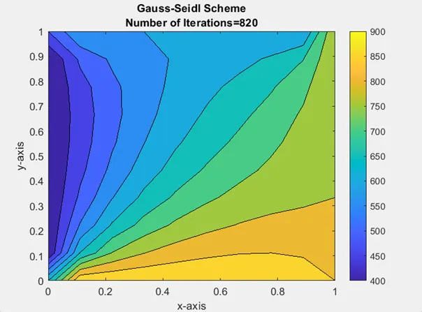
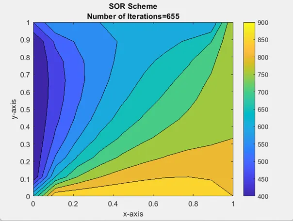
For Steady State,
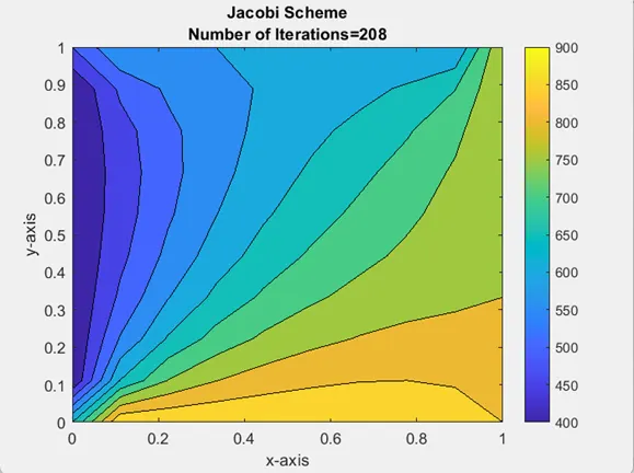
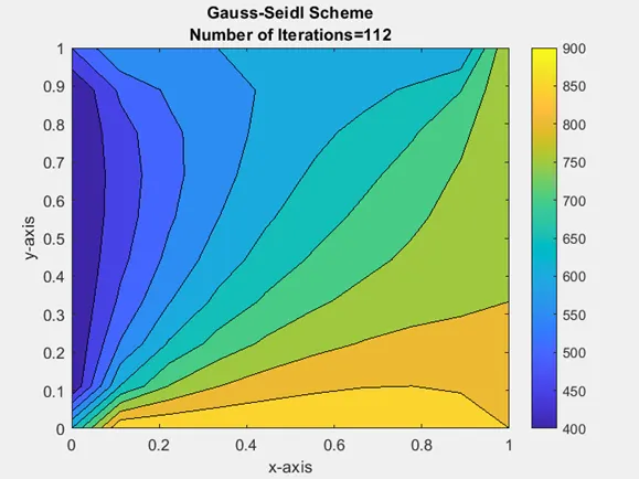
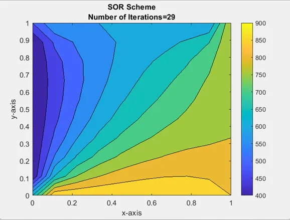
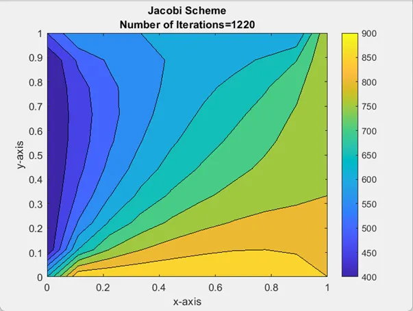
For Transient State (Implicit),
For Transient State (Explicit),
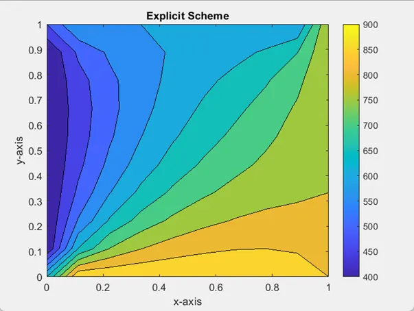
The solution converges the quickest for SOR (with an appropriately chosen relaxation factor), then for Guss-Seidl and the least for Jacobi, for both the transient and steady state analysis.