Week 5.1 - Mid term project - Solving the steady and unsteady 2D heat conduction problem
Aim: Solving the steady and unsteady 2D heat conduction problem using MATLAB.
Objective:
- Solve the2D heat conduction equation by using the point iterative techniques that were taught in the class.
- To write code for both implicit and explicit schemes (This is for the transient analysis only).
- Compare the convergence rate [Number of iterations] of the steady state and transient [explicit and implicit] simulations and justify the numerics.
- To implement the following methods for solving implicit equations.
- Jacobi
- Gauss-seidel
- Successive over-relaxation
Given Data:
- Top Boundary = `600 K`
- Bottom Boundary = `900 K`
- Left Boundary = `400 K`
- Right Boundary = `800 K`
- Error Criteria = `1^(e-4)`
Theory:
- A generalized conduction equation is given
- `(del^2T)/(delx^2)+(del^2T)/(dely^2)+(del^2T)/(delz^2)+q/k=1/alpha (delT)/(del tau)`
- Where, `T` = Temperature
`q` = Heat Genearated
`alpha` = Thermal Diffusivity - Thermal diffusivity is a thermophysical property of a material defined as the ratio of thermal conductivity of the material and its thermal capacity.
- For steady-state, time derivative is not considered, their fore below equation represents the 2D steady-state Heat conduction (elliptic).
- `((del^2T)/(delx^2) + (del^2T)/(dely^2)) = 0`
- `((del^2T)/(delx^2) + (del^2T)/(dely^2)) = 0`
- Steady state 2D heat condistion
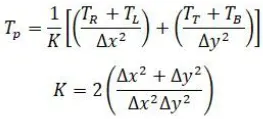
- Transient 2D heat conduction (Explicit)
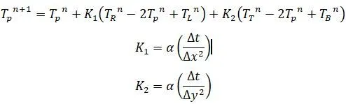
- Transient 2D heat conduction (Implicit)
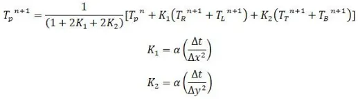
Matlab Code:
- Steady-State 2D Heat conduction
clear all close all clc % Domain and dicretization length number_node = 10; domain_length = 1; %Value of x and y at nodes in a discretization plane x = linspace(0,domain_length,number_node); y = linspace(0,domain_length,number_node); dx = domain_length/(number_node-1); dy = domain_length/(number_node-1); %Let define a temperature value at all nodes with initial guess 300k T = 300*ones(number_node,number_node); %Initia boundary conditions at left and right T(1:end,1) = 400; T(1:end,end) = 800; %Initia boundary conditions at bottom and top T(end,1:end) = 900; T(1,1:end) = 600; %Average values of T at boundaries T(1,1) = 500; T(end,1) = 650; T(1,end) = 700; T(end,end) = 850; %Temperature value to compute T_old = T; %Constant value K = (2*(dx^2+dy^2))/(dx^2*dy^2); omegha = 1.2; %Random error value while loop initalize error = 10; tol = 1e-4; no_iteration = 0; method = input('Enter(1) for jacobi,(2) for gauss seidel,(3) for sos'); if method == 1 while(error>tol) for i = 2:number_node-1 for j = 2:number_node-1 term1 = (T_old(i+1,j)+T_old(i-1,j))/dx^2; term2 = (T_old(i,j+1)+T_old(i,j-1))/dy^2; T(i,j) = (term1+term2)/K; end end error = max(max(abs(T_old-T))); %To upadte previous velcity with new velocity %The iteration T_old = T; no_iteration = no_iteration+1; end elseif method == 2 while(error>tol) for i = 2:number_node-1 for j = 2:number_node-1 term1 = (T_old(i+1,j)+T(i-1,j))/dx^2; term2 = (T_old(i,j+1)+T(i,j-1))/dy^2; T(i,j) = (term1+term2)/K; end end error = max(max(abs(T_old-T))); %To upadte previous velcity with new velocity %The iteration T_old = T; no_iteration = no_iteration+1; end else while(error>tol) for i = 2:number_node-1 for j = 2:number_node-1 term1 = (T_old(i+1,j)+T(i-1,j))/dx^2; term2 = (T_old(i,j+1)+T(i,j-1))/dy^2; T(i,j) = ((1-omegha)*T_old(i,j))+(omegha*((term1+term2)/K)); end end error = max(max(abs(T_old-T))); %To upadte previous velcity with new velocity %The iteration T_old = T; no_iteration = no_iteration+1; end end %To visualize a result [X,Y] = meshgrid(x,y); contourf(X,Y,T) colorbar set(gca,'ydir','reverse') - Unsteady-State 2D Heat conduction
clear all close all clc % Domain and dicretization length number_node = 10; domain_length = 1; %value of x and y at nodes in a discretization plane x = linspace(0,domain_length,number_node); y = linspace(0,domain_length,number_node); dx = (domain_length/number_node-1); dy = (domain_length/number_node-1); dt = 1/10; %Let define a temperature value at all nodes with initial guess 300k T = 300*ones(number_node,number_node); % Initia boundary conditions at left and right T(1:end,1) = 400; T(1:end,end) = 800; % Initia boundary conditions at bottom and top T(end,1:end) = 900; T(1,1:end) = 600; %average values of T at corner boundaries T(1,1) = 500; T(end,1) = 650; T(1,end) = 700; T(end,end) = 850; %Temperature value to compute for previous space terms T_old = T; % copy of T for previous time_step T_prev = T; %constants alpha = 1.5; omegha = 1.15; K1 = (alpha*dt)/(dx^2); K2 = (alpha*dt)/(dy^2); iteration = 0; approach = input('Enter 1 for implicit or Enter 2 for explicit') if approach == 1 method = input('Enter 1 for jacobi or 2 for gauss seidel or 3 for sos') if method == 1 for nt = 1:1500 error = 10; tol = 1e-4; while(error>tol) for i = 2:number_node-1 for j = 2:number_node-1 term1 = 1/(1+(2*K1)+(2*K2)); term2 = K1*(T_old(i+1,j)+T_old(i-1,j)); term3 = K2 *(T_old(i,j+1)+T_old(i,j-1)); T(i,j) = term1*(T_prev(i,j)+term2+term3); end end iteration = iteration+1; error = max(max((abs(T_old-T)))); T_old = T; end T_prev = T; end elseif method ==2 for nt = 1:1500 error = 10; tol = 1e-4; while(error>tol) for i = 2:number_node-1 for j = 2:number_node-1 term1 = 1/(1+(2*K1)+(2*K2)); term2 = K1*(T_old(i+1,j)+T(i-1,j)); term3 = K2 *(T_old(i,j+1)+T(i,j-1)); T(i,j) = term1*(T_prev(i,j)+term2+term3); end end iteration = iteration+1; error = max(max(abs(T_old-T))); T_old = T; end T_prev = T; end else for nt = 1:1500 error = 10; tol = 1e-4; while(error>tol) for i = 2:number_node-1 for j = 2:number_node-1 term1 = 1/(1+(2*K1)+(2*K2)); term2 = K1*(T_old(i+1,j)+T(i-1,j)); term3 = K2 *(T_old(i,j+1)+T(i,j-1)); term4 = term1*(T_prev(i,j)+term2+term3); T(i,j)=(1-omegha)*T_old(i,j)+(omegha*term4); end end iteration = iteration+1; error = max(max(abs(T_old-T))); T_old = T; end T_prev = T; end end else for nt = 1:1500 for i = 2:number_node-1 for j = 2:number_node-1 term1 = K1*(T_prev(i+1,j)-2*T_prev(i,j)+T_prev(i-1,j)); term2 = K2*(T_prev(i,j+1)-2*T_prev(i,j)+T_prev(i,j-1)); T(i,j) = T_prev(i,j)+term1+term2; end end % to upadte the previous timestep value with new timestep value %got from the iteration T_prev = T; iteration = iteration+1; end end %To visualize the result [X,Y] = meshgrid(x,y); figure(1) contourf(X,Y,T) colorbar set(gca,'ydir','reverse')
Result:
-
Steady-State analysis
- Jacobi
Enter(1) for jacobi,(2) for gauss seidel,(3) for sos 1 >> no_iteration no_iteration = 207 >> - Gauss- Siedel
Enter(1) for jacobi,(2) for gauss seidel,(3) for sos 2 >> no_iteration no_iteration = 111 >> - Successive over relaxation
Enter(1) for jacobi,(2) for gauss seidel,(3) for sos 3 >> no_iteration no_iteration = 75 >>
- Jacobi
-
Transient analysis
- Jacobi
Enter 1 for implicit or Enter 2 for explicit 1 approach = 1 Enter 1 for jacobi or 2 for gauss seidel or 3 for sos 1 method = 1 >> iteration iteration = 3421 >> - Gauss- Siedel
Enter 1 for implicit or Enter 2 for explicit 1 approach = 1 Enter 1 for jacobi or 2 for gauss seidel or 3 for sos 2 method = 2 >> iteration iteration = 2893 >> - Successive over-relaxation
Enter 1 for implicit or Enter 2 for explicit 1 approach = 1 Enter 1 for jacobi or 2 for gauss seidel or 3 for sos 3 method = 3 >> iteration iteration = 2554 >> - Xplicit
According to CFL stability criteria, K1+K2<0.5.
Enter 1 for implicit or Enter 2 for explicit 2 approach = 2 >> iteration iteration = 1500 >> K1+K2 ans = 0.3704 >>
- Jacobi
Explanstion:
- Steady-State 2D Heat conduction
- First inputs are defined into variables and the temperature array is created.
- Boundary conditions are introduced into the temperature array, and at corners, boundary values are averaged.
- Constants like alpha, omega, tolerance are defined to run the iteration.
- Input must be provided by the user, to choose the iterative method.
- The if-else loop is used to solve the equation using the selected(input from the user) iterative technique.
- while loop is used to run the iterative technique till the required accuracy is achieved.
- Two for loop is used to calculate the temperature values at every node at each iterative step.
- Unsteady-State 2D Heat conduction
- Inputs are defined into variables and the temperature array is created.
- Boundary conditions are introduced into the temperature array, and at corners, boundary values are averaged.
- Constants like alpha, omega, tolerance are defined to run the iteration.
- Here a user must provide, one or two inputs.
- The first input is to whether solve the problem using an explicit approach or an implicit approach.
- If an implicit approach is selected, then the user must provide another input, to select the iterative technique.
- Here we are going to understand the concept of the 2d heat conduction equation of both stead and transient state of flow. We need to understand the derivation part where the terms are being discretized sequentially and then we move on to the coding part. There are few things that need to be considered before going over it is that for steady-state we need to apply iterative solvers and for transient, we have to solve both the schemes we seen in the previous section as IMPLICIT and EXPLICIT.
Output:
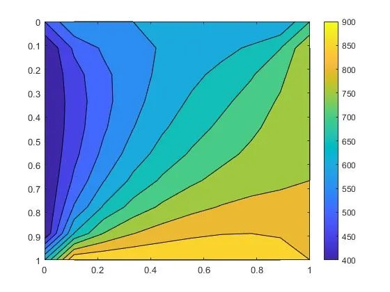
Conclusion:
- It can be concluded that the number of iteration required is least in SOR method. The maximum number of iteration is seen in jacobi method. So, the trend in terms of the number of iteration for convergence is :
Jacobi method > Gauss-siedel method > SOR method. - From above simulation we can see explicit method is converging faster than implicit methods taking less time for simulations. For steady state we can opt for SOR method as it reaches converge faster than any other methods.
- Between Explicit and Implicit results, the latter one does not depend greatly on Courant number for its stability and convergence, on the other hand in the Explicit approach information from a given cell or mesh element must propagate to its immediate neighbours, hence the low CFL number needs to be considered.