Week 5.1 - Mid term project - Solving the steady and unsteady 2D heat conduction problem
Aim: Solve the 2D heat conduction equation using the point iterative techniques. The Boundary conditions for the problem are as follows;
Top Boundary = 600 K
Bottom Boundary = 900 K
Left Boundary = 400 K
Right Boundary = 800 K
The following methods for solving implicit equations.
- Jacobi
- Gauss-seidel
- Successive over-relaxation
Your absolute error criteria are 1e-4
Introduction:
Explicit Method
When a direct computation is made for an unknown quantity in terms of a known quantity. This computation is called Explicit. This method requires stability criteria which when satisfied leads to a stable solution. Because of the stability criteria, small time steps have to be taken to obtain stable solutions. With the decrease in time step, the number of computations increases, and hence the computational time required for the solution to converge is less, and the accuracy of the solution is high.
Implicit Method
When a computation is made for a dependent variable defined by a set of equations and a matrix is involved to find the unknown variable. This computation is called the Implicit method. This method is unconditionally stable as a result, no stability criteria are required to obtain a stable result and the computational time required for the solution to converge is high and the accuracy of the solution is less relative to the explicit method because this method uses simultaneous equations and uses guess values as the initial values to find the approximated values. If the guess values are closer to the desired value the computation time is less. As there is no stability criteria requirement larger time steps can be used.
Let's define what are the iterative techniques we are using here:
2D Heat Conduction Equation:
`(delT)/(delt) = alpha*((del^2T)/(delx^2) + (del^2T)/(dely^2))`
The time derivative term `(delT)/(delx)` is hyperbolic in nature which can be discretized using a forward differencing scheme and the spatial derivatives are elliptical in nature which can be discretized using a central differencing scheme.
Discretization of Time derivative using forward difference scheme since the time derivative is varying in time direction which can be solved by marching method.
`((delT)/(delt))_(i,j)^n = (T_(i,j)^(n+1) - T_(i,j)^n)/(Deltat) + 0(Deltat)`
Discretization of spacial derivatives using central differencing scheme since the spatial derivatives are elliptical in nature, which uses information from neighboring points to obtain a solution. Below are the discretization for x and y spatial derivatives.
`((del^2T)/(delx^2))_(i,j)^n = (T_(i+1,j)^(n) - 2T_(i,j)^n + T_(i-1,j)^(n))/(Deltax)^2 + 0(Deltax^2)`
`((del^2T)/(dely^2))_(i,j)^n = (T_(i,j+1)^(n) - 2T_(i,j)^n + T_(i,j-1)^(n))/(Deltay)^2 + 0(Deltay^2)`
From the PDE heat conduction equation,
`(T_(i+1,j)^(n) - 2T_(i,j)^n + T_(i-1,j)^(n))/(Deltax)^2 + (T_(i,j+1)^(n) - 2T_(i,j)^n + T_(i,j-1)^(n))/(Deltay)^2 = 1/alpha (T_(i,j)^(n+1) - T_(i,j)^n)/(Deltat)`
where n is the current time step and n+1 is the next time step.
i, i+1 are the neighboring points in the x direction, and j, j+1 is the neighboring points in the y direction.
`Deltax` is grid spacing in the x direction. `Deltay` is grid spacing in the y direction.
Iterative Solver:
1. Jacobi iterative solver:
In this method, the temperature at n+1th iteration is found using old values of the temperature defined at nth iterations. Using the approximation obtained iterations procedure it continued until the desired accuracy of the solution is obtained.
2. Gauss-Seidel iterative solver:
In this type of iterative solver, the temperature at n+1 iterations uses values of n+1 iterations that have already been computed. In this way, old approximated values are overwritten with new approximate values for the iterations performed. Unlike Jacobi, Gauss seidel requires one storage vector which can be overwritten with each computation. This helps the solution to cover faster than the Jacobi method.
3. Successive over-relaxation iterative solver.
In this type of iterative solver relaxation factor is used which helps increase the convergence rate. It goes by the formula
`T^(n+1) = T^n*(1-omega) + omega* T(GS) or T(Jacobi)`
where `omega` is the relaxation factor. Its range is from 0<`omega`<2
when `omega` is between 0-1 it is called under relaxed state.
This condition is used when the temperature gradient is high and due to this condition, the time step does not overshoot and helps to converge at a faster rate.
when `omega` is between 1-2 it is called over the relaxed state.
This condition is used when the temperature gradient is low and due to this condition, larger time steps are used to obtain the steady state i.e., for the values to converge at a faster rate.
`T^n` is the value of temperature for previous iterations
T(GS) or T(Jacobi) is the temperature of value for n+1th iteration using gauss seidel or Jacobi iterative solver.
Steady State 2D Heat Conduction Equation :
Steady-state is where the fluid properties do not change with respect to time.
From the 2D heat conduction equation since the system is in a steady state time derivative is zero and diffusivity is constant.
`(delT)/(delt) = 0`
Hence we the equation for the steady state as:
`((del^2T)/(delx^2) + (del^2T)/(dely^2)) = 0;`
Discretization for Steady State:
`(T_L - 2*T_P + T_R)/(Deltax^2) + (T_T - 2*T_P + T_B)/(Deltay^2) = 0;`
`T_P = T_(i,j)`
`T_L = T_(i-1,j)`
`T_R = T_(i+1,j)`
`T_T = T_(i,j+1)`
`T_B = T_(i,j-1)`
Solving for T(i, j), we get
`T_P = K_1(T_L + T_R) + K_2(T_T + T_B)`
`K_1 = (Deltay^2)/(2*(Deltax^2 + Deltay^2)`
`K_2 = (Deltax^2)/(2*(Deltax^2 + Deltay^2)`
Solving the 2D Steady Heat Conduction equation implicitly.
The formula for Jacobi iterative solver
`(T_P)^(n+1) = K_1(T_L + T_R)^n + K_2(T_T + T_B)^n`
The formula for Gauss-Seidel Iterative Solver
`(T_P)^(n+1) = K_1(T_L + T_R)^(n+1) + K_2(T_T + T_B)^(n+1)`
The formula for Successive over-relaxation iterative solver
`(T_P)^(n+1) = T_P^n*(1-omega)+ omega*(K_1(T_L + T_R)^(n+1) + K_2(T_T + T_B)^(n+1))`
Transient state:
An unsteady state is where the fluid properties change with respect to time.
The formula for the 2D transient heat conduction equation is
`(delT)/(delt) = alpha*((del^2T)/(delx^2) + (del^2T)/(dely^2))`
Discretization for Unsteady State heat conduction equation:-
`(T_P^(n+1) - T_P^n)/(Deltat) - alpha*((T_L - 2*T_P + T_R)/(Deltax^2) + (T_T - 2*T_P + T_B)/(Deltay^2)) = 0;`
`T_P = T_(i,j)`
`T_L = T_(i-1,j)`
`T_R = T_(i+1,j)`
`T_T = T_(i,j+1)`
`T_B = T_(i,j-1)`
Solving the 2D transient heat conduction equation explicitly we get,
`T_P^(n+1) = (1-2*K_1-2*K_2)*T_P^n + K_1(T_L + T_R)^n + K_2(T_T + T_B)^n`
`K_1 = alpha*(Deltat)/(Deltax^2)`
`K_2 = alpha*(Deltat)/(Deltay^2)`
Stability Criteria
`K_1 + K_2 <= 0.5` Stability criteria for 2D heat conduction equation when solving explicitly.
Solving for the 2D Transient Heat Conduction equation implicitly we get,
`(T_P)^(n+1) = 1/K*[T_P^n+ K_1(T_L + T_R)^(n+1) + K_2(T_T + T_B)^(n+1)]`
`K = 1+2*K_1 + 2*K_2`
`K_1 = alpha*(Deltat)/(Deltax^2)`
`K_2 = alpha*(Deltat)/(Deltay^2)`
here n+1 is the next time step and n is the preceding time step.
Formula for jacobi iterative solver
`T_P^(n+1) = (T_P^n + K_1*(T_L^n + T_R^n) + K_2*(T_T^n + T_B^n))/(1 + 2*K_1 + 2*K2)`
The formula for Gauss seidel
`T_P^(n+1) = (T_P^n + K_1*(T_L^(n+1) + T_R^n) + K_2*(T_T^n + T_B^(n+1)))/(1 + 2*K_1 + 2*K2)`
The formula for Successive over relaxation
`T_P^(n+1) = T_P^n*(1-omega) + omega*[(T_P^n + K_1*(T_L^(n+1) + T_R^n) + K_2*(T_T^n + T_B^(n+1)))/(1 + 2*K_1 + 2*K2)]`
Explanation
1. Specifying the number of grid points in the spacial domain x and y direction. In this case, is 10 grid points in the x and y directions.
2. Specify the length of the domain in the x and y space domain.
3. Defining the spacial domain for the length and grid points specified.
4. Calculating the grid spacing in the x and y space domain.
5. Defining temperature with the guess values 300K for the number of the grid points defined.
6. Applying the Boundary Conditions as mentioned in the problem.
7. The accuracy of the solution is measured with a computed approximated solution and compared with the tolerance value so that the converged solution is in the desired accuracy.
8. A copy of the initial temperature matrix is made in told and t_pre which is used while calculating the temperature values of n+1 time steps explicitly and implicitly.
9. Calculating `K, K_1, and K_2` Here `alpha` is taken 1.4.
10. Function is called to calculate the temperature values at n+1 time step for both steady and unsteady state using different iterative solvers and explicit method is also used for calculating temperature for unsteady state heat conduction equation.
Matlab Program:
%Code to study the behaviour of steady state and transient state analysis
%using explicit and implicit method.
clear all
close all
clc

%Defining spacial domain
nx = 10;ny=10;
%Specifying length of the domain.
L=1;
%defining space domain
x = linspace(0,L,nx);
y = linspace(0,L,ny);
%grid size
dx = x(2)-x(1);
dy = y(2)-y(1);

%defining temperature
t = 300*ones (nx,ny);
% [t] = 300*meshgrid(x,y);
t(1:end,1)=400;%<-- left boundary
t(end,1:end)=900;%<-- bottom boundary
t(1,1:end)=600;%<-- top boundary
t(1:end,end)=800;%<-- right boundary
% Edge temperature
t(1,1)= (t(1,2)+t(2,1))/2;
t(end,1) = (t(end,2)+t((end-1),1))/2;
t(1,end)= (t (1,(end-1))+t(2,end))/2;
t(end,end)=(t((end-1),(end))+ t(end,(end-1)))/2;

%tolerance
tol=1e-4;

%Making a copy of the initial temperature matrix.
told=t;
t_pre=t;

%Coefficient obtained from the derivation for steady state equation
k = 2*(dx^2+dy^2)/(dx^2*dy^2);

%diffusivity co-efficient in the  2D heat conduction equation
alpha = 1.4;

% Calculation of time step
dt = (0.5)/((alpha/dx^2)+(alpha/dy^2));

% Co-efficient  multipied for x diffuse term
k1 = dt*alpha/dx^2;
% Co-efficient  multipied for y diffuse term
k2 = dt*alpha/dy^2;

%relaxation factor for successive over relaxation facotr for steady state
%heat conduction.
a = 1.5;
%relaxation factor for Successive over relaxation factor for transiet heat
%conduction
a1 = 1.15;

%Function to calculate the temperature of Steady state using jacobi iterative solver
[error_j,iter1] = jacobi(nx,ny,t,told,k,dx,dy,tol);
%Function to calculate the temperature of Steady state using Gauss Seidal iterative solver
[error_gs,iter2] = gs(nx,ny,t,told,k,dx,dy,tol);
%Function to calculate the temperature Steady state using Successive over relaxation iterative solver
[error_sor_gs,iter3] = sor_gs(nx,ny,t,told,k,dx,dy,tol,a);
%Function to calculate the temperature of Transient heat conduction explicitly
[error_dt,iter_dt]=transient_heat_conduction(nx,ny,k1,k2,told,t,tol);
%Function to calculate the temperature of Unsteady state using jacobi iterative solver
[error_jac,iter_jac]=transient_heat_conduction_jacobi(nx,ny,k1,k2,told,t,tol,t_pre);
%Function to calculate the temperature of Unsteady state using Gauss Seidal iterative solver
[error_gs_imp,iter_gs_imp]=transient_heat_conduction_gs(nx,ny,k1,k2,told,t,tol,t_pre);
%Function to calculate the temperature of Unsteady state using Successive over relaxation iterative solver
[error_sor_gs_imp,iter_sor_gs_imp]=transient_heat_conduction_sor_gs(nx,ny,k1,k2,told,t,tol,t_pre,a1);
Explanation of Functions defined in the main script:
In the functions, a dummy error is assigned to the error variable so that the while loop condition would satisfy it and iterations are calculated.
The error is calculated and updated for each iteration. The error calculated is coded to take only the absolute values since negative values will not satisfy the while loop condition and iterations will be stopped and the results obtained will not be a converged result.
The number of iterations taken for the solution to converge is stored in the iter variable. This is done by incrementing the iter variable by 1 for each iteration.
As the iteration proceeds to calculate the temperature at n+1 time step temperature at the nth time step is required and these temperature values should be updated for each iteration. If the temperature values are not updated for each iteration the solution will not converge and the while loop will run infinite times.
Contourf plot is used to check if the solutions are converged or not i.e., the plot does not change as the approximated temperature value changes in the order of tolerance value defined. told stores the temperature values of the preceding time step, and t stores the temperature values of the n+1 time step.
This logic is used in the below functions to calculate the temperature of the Steady-state Heat Conduction equation for the desired accuracy.
Functions are as follows:
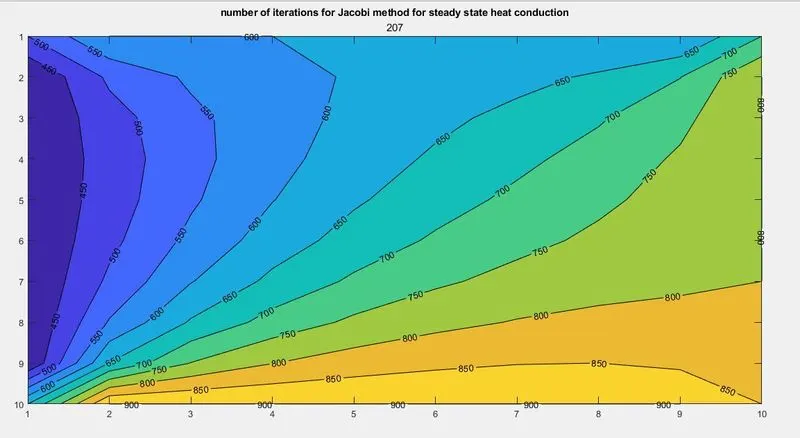
Function to calculate the temperature of Steady-state using Jacobi iterative solver
%Function to calculate the temperature of Steady state using jacobi iterative solver
function [error_j,iter1] = jacobi(nx,ny,t,told,k,dx,dy,tol)

        %defining iteration variable to store and display the number of
        %iterations computed for the values to converge.
        iter1 = 0;
        % Dummy error value
        error_j = 9e9;

    %convergence loop
    while (error_j>tol)

                %Iteration loop
                for i = 2:(nx-1)

                    for j = 2:(ny-1)

                        %Formula to calculate the temperature at each grid
                        %point
                        t(i,j)= (1/k)*(((told((i-1),j)+told((i+1),j))/dx^2)+((told(i,(j+1))+told(i,(j-1)))/dy^2));

                    end
                end

                %error for each iteration
                error1 = abs(told-t);
                error_j = max(error1,[],'all');

                %updating the temperature values for the next iteration.
                told = t;

                %incrementing iter variable by 1 to display the no. of
                %iterations taken for the solution to converge.
                iter1 = iter1+1;
    end
                % Plot representing the converged results.
                figure(1)
                [C,h]=contourf(t);
                %Labelling the plot here C reperesents the temperature values and h rotates the temperature values as it moves.
                clabel(C,h);
                axis ij;
                title('number of iterations for Jacobi method for steady state heat conduction',iter1);


end
This function uses Jacobi iterative solver, temperature at n+1 time step is calculated using temperature at an nth time step.
Output Graph:
Function to calculate the temperature of Steady-state using Gauss Seidal iterative solver
%Function to calculate the temperature of Steady state using Gauss Seidal iterative solver

function [error_gs,iter2] = gs(nx,ny,t,told,k,dx,dy,tol)

         % Dummy error value
        error_gs = 9e9;
        %defining iteration variable to store and display the number of
        %iterations computed for the values to converge.
        iter2 = 0;

        %convergence loop
        while (error_gs>tol)

             %Iteration loop
            for i = 2:(nx-1)

                for j = 2:(ny-1)

                    %Formula to calculate the temperature at each grid
                    %point
                    t(i,j)= (1/k)*(((t((i-1),j)+t((i+1),j))/dx^2)+((t(i,(j+1))+t(i,(j-1)))/dy^2));

                end
            end

            %error for each iteration
            error1 = abs(told-t);

            error_gs = max(error1,[],'all');


            %updating the temperature values for the next iteration.
            told = t;

            %incrementing iter variable by 1 to display the no. of
            %iterations taken for the solution to converge.
            iter2 = iter2+1;
        end

            % Plot representing the converged results.
            figure(2)
            [C,h]=contourf(t);
            %Labelling the plot here C reperesents the temperature values and h rotates the temperature values as it moves.
            clabel(C,h);
            axis ij;
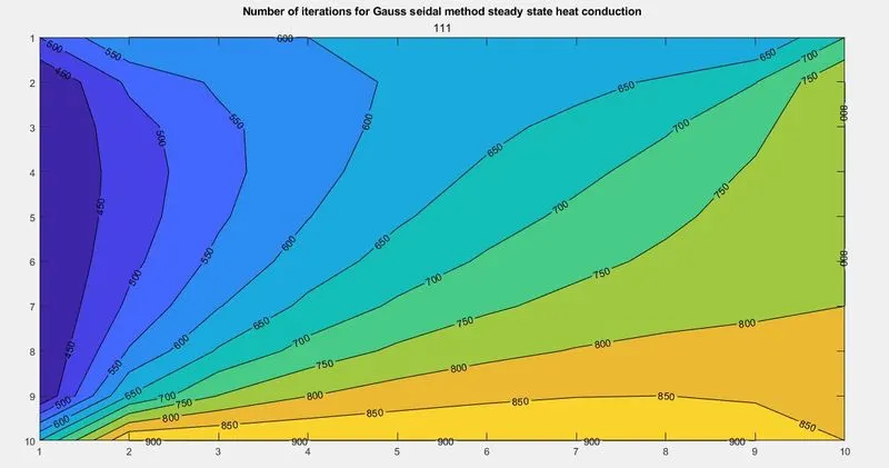
            title('Number of iterations for Gauss seidal method steady state heat conduction',iter2)

end
This function uses Gauss seidal iterative solver in which temperature at n+1 time step is calculated using n+1 approximated temperature in the previous iterations.
Output Graph:
Function to calculate the temperature of Steady-state using Successive over-relaxation iterative solver
%Function to calculate the temperature of Steady state using Successive over relaxation iterative solver
function [error_sor_gs,iter3] = sor_gs(nx,ny,t,told,k,dx,dy,tol,a)

   %Dummy error value
   error_sor_gs = 9e9;
   %defining iteration variable to store and display the number of
   %iterations computed for the values to converge.
   iter3 = 0;

   %Convergence loop
    while (error_sor_gs>tol)

            %iteration loop
            for i = 2:(nx-1)

                for j = 2:(ny-1)

                    %Formula to calculate the temperature at each grid
                    %point
                    t(i,j)= (1/k)*(((t((i-1),j)+told((i+1),j))/dx^2)+((told(i,(j+1))+t(i,(j-1)))/dy^2));

                    %Successive over relaxation Formula to calculate the
                    %temperature at each grid point.
                    t(i,j) = (told(i,j))*(1-a)+a*(t(i,j));

                end
            end

            %error for each iteration
            error1 = abs(told-t);

            error_sor_gs = max(error1,[],'all');

            %updating the temperature values for the next iteration.
            told = t;

            %incrementing iter variable by 1 to display the no. of
            %iterations taken for the solution to converge.
            iter3 = iter3+1;
    end
            % Plot representing the converged results.
            figure(3)
            [C,h]=contourf(t);
            %Labelling the plot here C reperesents the temperature values and h rotates the temperature values as it moves.
            clabel(C,h);
            axis ij;
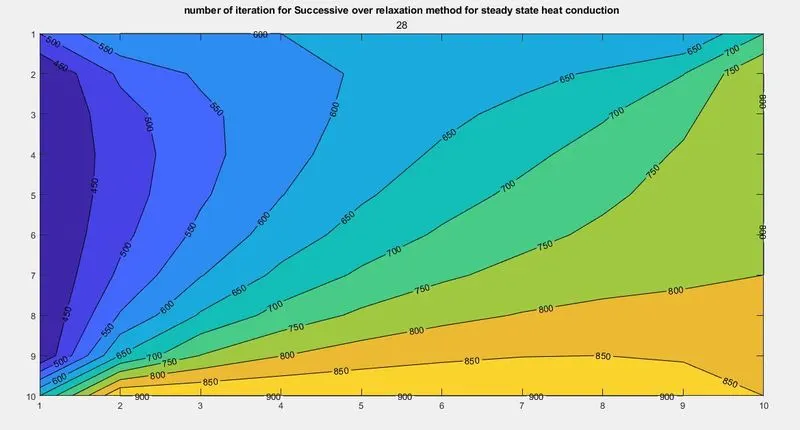
            title('number of iteration for Successive over relaxation method for steady state heat conduction', iter3)

end
This function uses Successive over-relaxation to calculate the temperature at the n+1 time step. It uses temperature values calculated using Gauss seidal method and relaxation factor which helps in increasing the convergence rate.
Output Graph:
Functions mentioned below use Unsteady state heat conduction equation formula to calculate the temperature values at the n+1 time step.
Function to calculate the temperature of an Unsteady state using an explicit method
%Function to calculate the temperature of Unsteady state using explicit
%method
function [error_dt,iter_dt]=transient_heat_conduction(nx,ny,k1,k2,told,t,tol)

    %dummy error
    error_dt = 9e9;
    %defining iteration variable to store and display the number of
   %iterations computed for the values to converge.
    iter_dt =0;
    %convergence loop
    while (error_dt>tol)

            %Iteration loop
            for i = 2:nx-1

                for j = 2:ny-1


                    H = told(i-1,j)-2*told(i,j)+told(i+1,j);%<-- This line represent temperature values in x direction
                    V = told(i,j-1)-2*told(i,j)+told(i,j+1);%<-- This line represent temperature values in y direction
                    %Formula to calculate the temperature at each grid
                    %point
                    t(i,j)= told(i,j)+k1*H+k2*V;


                end
            end

           %error for each iteration
            error1 = abs(told-t);
            error_dt = max(error1,[],'all');

            %updating the temperature values for the next iteration.
            told = t;

           %incrementing iter variable by 1 to display the no. of
           %iterations taken for the solution to converge.
           iter_dt = iter_dt+1;


    end
           %Plot representing the converged results.
           figure(4)
           [C,h]=contourf(t);
           %Labelling the plot here C reperesents the temperature values and h rotates the temperature values as it moves.
           clabel(C,h);
           axis ij
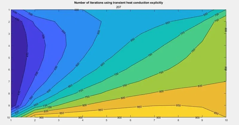
           title('Number of iterations using transient heat conduction explicitly',iter_dt);


end
Output Graph:
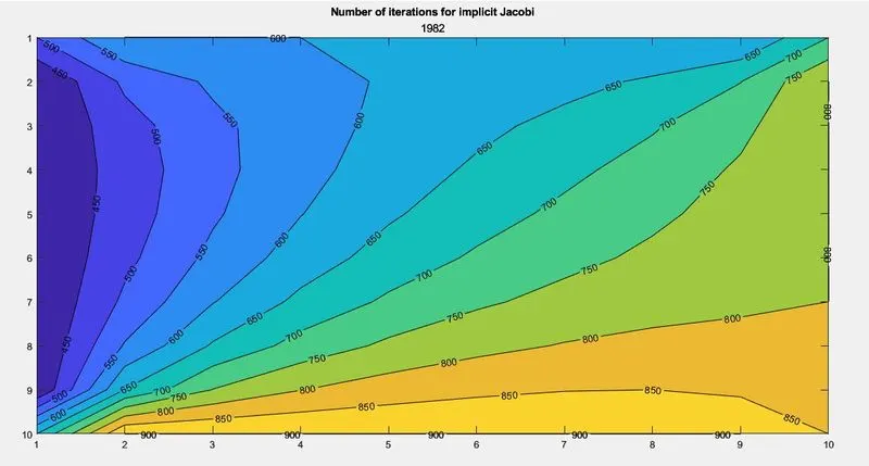
Function to calculate the temperature in an Unsteady state using Jacobi iterative solver
As we are now solving for the unsteady state heat conduction equation, a steady state is achieved after a certain number of time steps.
Hence 1st while loop is used to check for the steady state of the solution by calculating the error between temperature between successive time steps and comparing it with the tolerance values. At a steady state, the temperature values do not change with increases in the number of iterations and the error value reduces below the tolerance value. With this, the converging point is found.
2nd while loop functions in a similar way as 1st while loop. But in 2nd while loop it finds the converged value of temperature for the particular time step.
This logic is used in the below functions which are used to solve the 2D heat conduction equation implicitly.
%Function to calculate the temperature of Unsteady state using jacobi
%iterative solver
function [error_jac,iter_jac]=transient_heat_conduction_jacobi(nx,ny,k1,k2,told,t,tol,t_pre)

    % dummy error
    error_jac=9e9;
    error_f = 9e9;
   %defining iteration variable to store and display the number of
   %iterations computed for the values to converge.
    iter_jac=0;

    %While loop to stop iterations when the temperature values converge
    %whle computing for different time steps.
    while (error_f>tol)

        %Convergence loop each time step
        while (error_jac>tol)

                %Iteration loop
                for i = 2:nx-1

                    for j = 2:ny-1

                        %Co-efficient obtained while deriving for transient heat conduction equation
                        term1= (1+(2*k1)+(2*k2))^-1;
                        %k1 and k2 represent the cfl value for x and y
                        %domain repectively.
                        H = told(i-1,j)+told(i+1,j);%<-- This line represent temperature values in x direction
                        V = told(i,j-1)+told(i,j+1);%<-- This line represent temperature values in y direction
                        %Formula to calculate the temperature at each grid
                        %point
                        t(i,j)= (t_pre(i,j)*term1)+(term1*k1*H)+(term1*k2*V);


                    end
                end

                %error for each iteration
                error1 = abs(told-t);
                error_jac = max(error1,[],'all');
                %updating the temperature values for the next iteration.
                told = t;

                %incrementing iter variable by 1 to display the no. of
                %iterations taken for the solution to converge.
                iter_jac = iter_jac+1;


        end

      % error defined to obtain desired accuracy for the convergenc rate.
      error_f = max(max(abs(t_pre-t)));
      t_pre = t;
      %Reseting the error value for the covergence loop to compute for the
      %next time step.
      error_jac = 9e9;

    end

                %Plot representing the converged results.
                figure(5)
               [C,h]=contourf(t);
               %Labelling the plot here C reperesents the temperature values and h rotates the temperature values as it moves.
               clabel(C,h)
               axis ij
               title('Number of iterations for implicit Jacobi',iter_jac);


end
Output Graph:
Function to calculate the Temperature in an Unsteady state using Gauss seidal iterative solver.
%Function to calculate the temperature of Unsteady state using gauss seidal
%iterative solver
function [error_gs_imp,iter_gs_imp]=transient_heat_conduction_gs(nx,ny,k1,k2,told,t,tol,t_pre)

    %Definition of dummy error
    error_f = 9e9;
    error_gs_imp=9e9;
   %defining iteration variable to store and display the number of
   %iterations computed for the values to converge.
    iter_gs_imp=0;

    %While loop to stop iterations when the temperature values converge
    %whle computing for different time steps.
    while(error_f>tol)

        %Convergence loop each time step
        while (error_gs_imp>tol)

                %Iteration loop
                for i = 2:nx-1

                    for j = 2:ny-1

                        %Co-efficient obtained while deriving for transient heat conduction equation
                        term1= (1+(2*k1)+(2*k2))^-1;
                        %k1 and k2 represent the cfl value for x and y
                        %domain repectively.
                        H = t(i-1,j)+told(i+1,j);%<-- This line represent temperature values in x direction
                        V = t(i,j-1)+told(i,j+1);%<-- This line represent temperature values in y direction
                        %Formula to calculate the temperature at each grid
                        %point
                        t(i,j)= (t_pre(i,j)*term1)+(term1*k1*H)+(term1*k2*V);


                    end
                end

                %error for each iteration
                error1 = abs(told-t);
                error_gs_imp = max(error1,[],'all');

                %updating the temperature values for the next iteration.
                told = t;

               %incrementing iter variable by 1 to display the no. of
               %iterations taken for the solution to converge.
               iter_gs_imp = iter_gs_imp+1;


        end

      % error defined to obtain desired accuracy for the convergenc rate.
      error_f = max(max(abs(t_pre-t)));
      %Updating the previous temperature values to computed values.
      t_pre = t;
      %Reseting the error value for the covergence loop to compute for the
      %next time step.
      error_gs_imp = 9e9;

    end
                %Plot representing the converged results.
                figure(6)
               [C,h]=contourf(t);
               %Labelling the plot here C reperesents the temperature values and h rotates the temperature values as it moves.
               clabel(C,h)
               axis ij
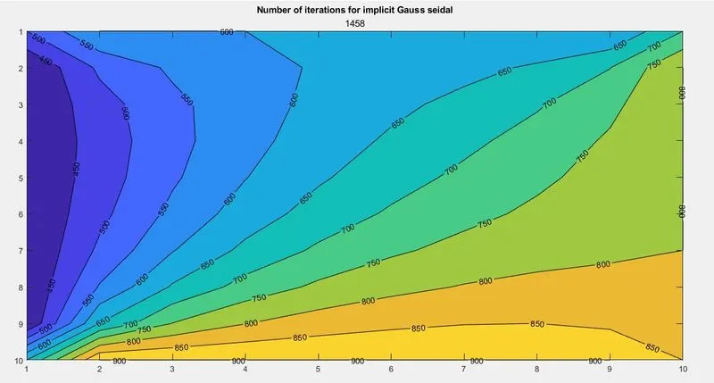
               title('Number of iterations for implicit Gauss seidal',iter_gs_imp);


end
Output Graph:
Function to calculate the temperature in an Unsteady state using a successive over-relaxation iterative solver
%Function to calculate the temperature of Unsteady state using successive
%over relaxation iterative solver
function [error_sor_gs_imp,iter_sor_gs_imp]=transient_heat_conduction_sor_gs(nx,ny,k1,k2,told,t,tol,t_pre,a1)

        %Definition of dummy error
        error_f = 9e9;
        error_sor_gs_imp = 9e9;
        %defining iteration variable to store and display the number of
         %iterations computed for the values to converge.
        iter_sor_gs_imp =0;

    %While loop to stop iterations when the temperature values converge
    %whle computing for different time steps.
    while (error_f>tol)

        %Convergence loop each time step

        while (error_sor_gs_imp>tol)

                %Iteration loop
                for i = 2:nx-1

                    for j = 2:ny-1
                        %Co-efficient obtained while deriving for transient heat conduction equation
                        term1= (1+(2*k1)+(2*k2))^-1;
                        H = t(i-1,j)+told(i+1,j);%<-- This line represent temperature values in x direction
                        V = t(i,j-1)+told(i,j+1);%<-- This line represent temperature values in y direction
                        %Formula to calculate the temperature at each grid
                        %point
                        t(i,j)= (t_pre(i,j)*term1)+(term1*k1*H)+(term1*k2*V);
                        %Successive over relaxation Formula to calculate the
                        %temperature at each grid point.
                        t(i,j)= (told(i,j))*(1-a1)+ a1*t(i,j);


                    end
                end

               %error for each iteration
               error1 = abs(told-t);
               error_sor_gs_imp = max(error1,[],'all');

               %updating the temperature values for the next iteration.
               told = t;

                %incrementing iter variable by 1 to display the no. of
               %iterations taken for the solution to converge.
               iter_sor_gs_imp = iter_sor_gs_imp+1;


        end

      %error defined to obtain desired accuracy for the convergenc rate.
      error_f = max(max(abs(t_pre-t)));
      %Updating the previous temperature values to computed values.
      t_pre = t;
      %Reseting the error value for the covergence loop to compute for the
      %next time step.
      error_sor_gs_imp = 9e9;

    end
               %Plot representing the converged results.
               figure(7)
               [C,h]=contourf(t);
               %Labelling the plot here C reperesents the temperature values and h rotates the temperature values as it moves.
               clabel(C,h)
               axis ij
               title('Number of iteration for implicit SOR',iter_sor_gs_imp);


end
Output Graph:
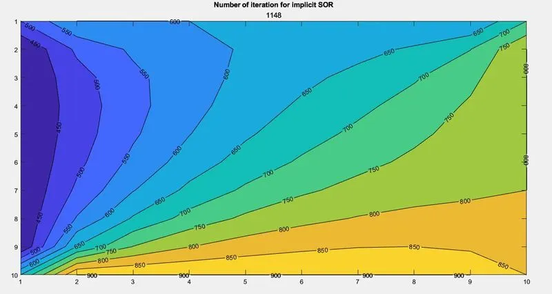
The above plots show the number of iterations required by the iterative solver to obtain the desired accurate solution.
Inference from the Plots:
The successive over-relaxation iterative solver convergence rate is higher than the Jacobi and gauss seidal method for both steady and unsteady state heat conduction equations. The number of iterations required by the successive over-relaxation method is less compared to Jacobi and gauss seidal method.
| Steady State Heat Conduction Equation | |
| Iterative Solver | No. of iterations |
| Jacobi | 207 |
| Gauss Seidal | 111 |
| Successive over Relaxation | 28 |
| Unsteady State Heat Conduction Equation. | |
| Iterative Solver | No. of iterations |
| Jacobi | 1982 |
| Gauss Seidal | 1458 |
| Successive over Relaxation | 1148 |
Conclusion:
The implicit method can be used for problems when converged results are needed in less computation time as they are unconditionally stable. With increases in time step size, the convergence rate is increased which leads to a steady state with less no. of iterations.
Explicit method results time accurate solutions as it is governed by stability criteria when not satisfied it leads to an unstable solution and requires more iterations to attain a steady state.
But in the code provided above time step size remains constant which is calculated with respect to the stability criteria. Hence for this time step size, the explicit scheme leads to a faster convergent rate, and as the time step size is small the number of iterations increases for the implicit scheme which results in a slower convergence rate.