Week 5.1 - Mid term project - Solving the steady and unsteady 2D heat conduction problem

Aim : To Solve the 2D heat conduction equation by using the point iterative techniques . The Boundary conditions for the problem are as follows

Steady state 2D heat conduction :steady state analysis is done at a constant temperature

`(d^2T)/dx^2+(d^2T)/dy^2`=0

the equation to find solution `T_p=1/k(frac(T_L+T_R)(Deltax^2))+1/k(frac(T_T+T_B)(Deltay^2))`

the given boundary conditions,

Top Boundary = 600 K

Bottom Boundary = 900 K

Left Boundary = 400 K

Right Boundary = 800 K

for solving implicit equations using iterations methods,

1. Jacobi

2. Gauss-seidel

3. Successive over-relaxation

coding :

Main code :

close all
clear 
clc

% inputs 
nx=10;  % no of nodes 
ny=10;  % no of nodes
x=linspace(0,1,nx);
y=linspace(0,1,ny);
dx=x(2)-x(1);
dy=y(2)-y(1);
tolerance=1e-4;
T=300*ones(ny,nx);
% Boundary conditions
T(:,1)=400;
T(1,:)=600;
T(ny,:)=900;
T(:,nx)=800;
% implementing corner conditions
T(1,1)=(600+400)/2;
T(ny,1)=(400+900)/2;
T(1,nx)=(600+800)/2;
T(ny,nx)=(800+900)/2;

%T_initial=T;
T_old=T;
k=2*((dx^2+dy^2)/(dx^2*dy^2));
omega=1.4;
[T_jacobi,iteration_jacobi] = steady_jacobi(nx,ny,dx,dy,k,T,tolerance,T_old);
[T_gauss,iteration_gauss] = steady_gausssiedal(nx,ny,dx,dy,k,T,tolerance,T_old);
[T_sor,iteration_sor] = steady_sor(nx,ny,dx,dy,k,T,omega,tolerance,T_old);
% ploting
figure(1)
contourf(x,y,T_jacobi,ShowText="on");
set(gca,'ydir','reverse')
colormap(jet)
colorbar
title('jacobi_iterative_method')
xlabel('x-axis')
ylabel('y-axis')
pause(0.01)

figure(2)
contourf(x,y,T_gauss,ShowText="on");
set(gca,'ydir','reverse')
colormap(jet)
colorbar
title('guasssiedal_iterative_method')
xlabel('x-axis')
ylabel('y-axis')
pause(0.01)

figure(3)
contourf(x,y,T_sor,ShowText="on");
set(gca,'ydir','reverse')
colormap(jet)
colorbar
title('sor_iterative_method')
xlabel('x-axis')
ylabel('y-axis')
pause(0.01)

Function program for jacobi

function [T,j_iterations] = steady_jacobi(nx,ny,dx,dy,k,T,tolerance,T_old)

% jacobi method
%convergence loop
j_iterations=1;
error=100;
while (error>tolerance)
    %space loop
    for i=2:nx-1
        for j=2:ny-1
            H=T_old(i-1,j)+T_old(i+1,j);
            V=T_old(i,j-1)+T_old(i,j+1);
            T(i,j)=(1/k)*(H)/(dx^2)+(1/k)*(V)/(dy^2);
        end
    end
    j_iterations=j_iterations+1;
    error=max(max(abs(T_old-T)));
    T_old=T;
    
end
end

Function program for gausssiedal

function [T,g_iterations] = steady_gausssiedal(nx,ny,dx,dy,k,T,tolerance,T_old)

% jacobi method
%convergence loop
g_iterations=1;
error=100;
while (error>tolerance)
    %space loop
    for i=2:nx-1
        for j=2:ny-1
             H=T(i-1,j)+T_old(i+1,j);
             V=T(i,j-1)+T_old(i,j+1);
            T(i,j)=((H)/(dx^2)+(V)/(dy^2))/k;
        end
    end
    g_iterations=g_iterations+1;
    error=max(max(abs(T_old-T)));
    T_old=T;
    
end
end

Function program for SOR(success over relaxation)

function [T,s_iterations] = steady_sor(nx,ny,dx,dy,k,T,omega,tolerance,T_old)

% jacobi method
%convergence loop
s_iterations=1;
error=100;
while (error>tolerance)
    %space loop
    for i=2:nx-1
        for j=2:ny-1
            H=(T(i-1,j)+T_old(i+1,j))/(dx^2);
             V=(T(i,j-1)+T_old(i,j+1))/(dy^2);
            T(i,j)=(1-omega)*T_old(i,j)+(omega*(H+V))/k;
        end
    end
    s_iterations=s_iterations+1;
    error=max(max(abs(T_old-T)));
    T_old=T;
    
end
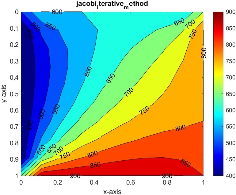
end

Result: In steady state jacobi iterative method

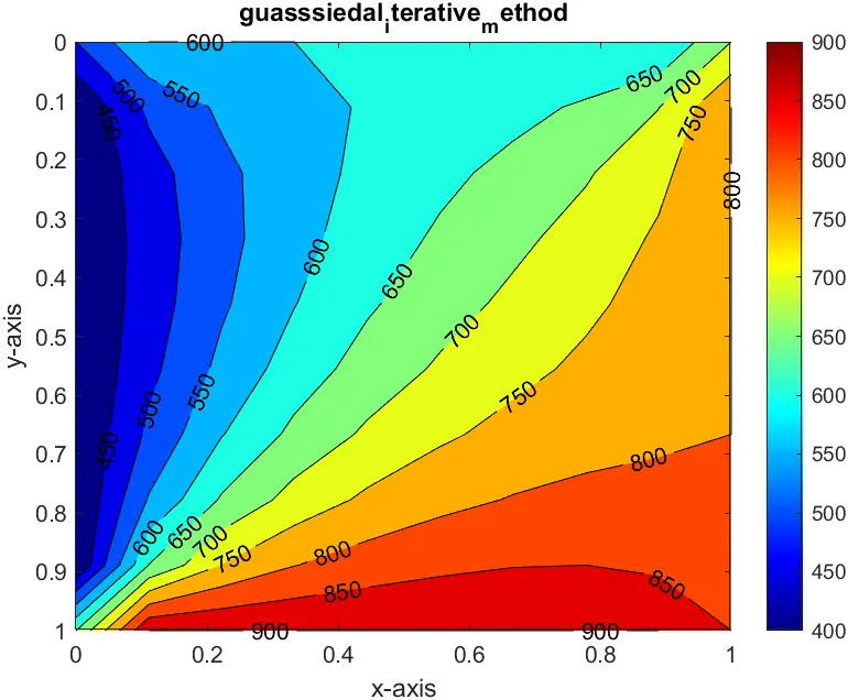
steady state gausssiedal iterative method:

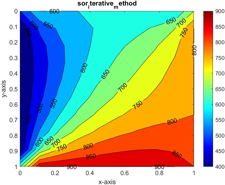
steady state SOR iterative method:

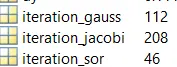
Iterations for jacobi : 208

Iterations for gausssiedal : 112

Iterations for SOR : 46

here we can see iterations are more in jacobi and gausssiedal less in SOR

Transient analysis : The time required to change from one state to another is called the transient time,the transient solution will converge to the steady-state solution over a long period of time.

Explicit method : When a direct computation of the dependent variables can be made in terms of known quantities, the computation is said to be explicit.

formula for transient explicit method : `T_p^(n+1)=T_p^n+k1(T_L-2T_P+T_R)^n+k2(T_T-2T_P+T_B)^n`

Implicit : When the dependent variables are defined by coupled sets of equations, and either a matrix or iterative technique is needed to obtain the solution, the numerical method is said to be implicit.

formula for transient implicit method : `(T_p^(n+1)-T_p^n)/(Deltat)=alpha(T_L-2T_p+T_R)/(Deltax^2)+(T_T-2T_p+T_B)/(Deltay^2)`

Now writing code for explicit method:

close all
clear
clc

% inputs 
nx=20;
ny=20;
x=linspace(0,1,nx);
y=linspace(0,1,ny);
dx=x(2)-x(1);
dy=y(2)-y(1);
tolerance=1e-4;
T=300*ones(ny,nx);
T(:,1)=400;
T(1,:)=600;
T(end,:)=900;
T(:,end)=800;
T(1,1)=(600+400)/2;
T(end,1)=(400+900)/2;
T(1,end)=(600+800)/2;
T(end,end)=(800+900)/2;
[xx,yy]=meshgrid(x,y);

Told=T;
dt=1e-4;
alpha=1.4;
k1=(alpha)*(dt/dx^2);
k2=(alpha)*(dt/dy^2);
cfl=k1+k2;
Explicit_iteration=1;

% Time loop
for nt=1:1400
    error=100;

    while(error>tolerance)
    for i=2:nx-1
        for j=2:ny-1
            H= k1*(Told(i-1,j)-2*Told(i,j)+Told(i+1,j));
            V= k2*(Told(i,j-1)-2*Told(i,j)+Told(i,j+1));
            T(i,j)= Told(i,j)+(H)+(V);
        end
    end
    error=max(abs(Told-T));
    Told=T;
    Explicit_iteration=Explicit_iteration+1;
    end
end

% Plotting
contourf(x,y,T,ShowText="on");
set(gca,'ydir','reverse')
colormap(jet)
colorbar
title('explicit_method')
xlabel('x-axis')
ylabel('y-axis')
 pause(0.01)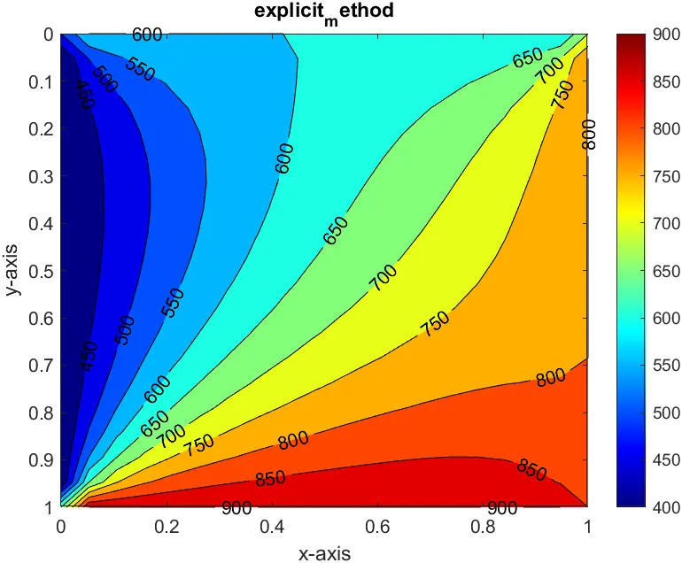

writing code for transient implicit method using iterations (jacobi,gausssiedal,sor)

main code :

close all
clear 
clc

% inputs 
nx=20;
ny=20;
x=linspace(0,1,nx);
y=linspace(0,1,ny);
dx=x(2)-x(1);
dy=y(2)-y(1);
tolerance=1e-4;
T=300*ones(nx,ny);
T(:,1)=400;
T(1,:)=600;
T(end,:)=900;
T(:,end)=800;
T(1,1)=(600+400)/2;
T(end,1)=(400+900)/2;
T(1,end)=(600+800)/2;
T(end,end)=(800+900)/2;

T_initial=T;
Told=T;
Tprev=T;
dt=1;
alpha=1.4;
omega=1.2;
k1=(alpha)*(dt/dx^2);
k2=(alpha)*(dt/dy^2);
[T_jacobi, iterations_jacobi] = transient_jacobi(nx,ny,k1,k2,Told,Tprev,tolerance,T);
[T_gausssiedal, iterations_gausssiedal] = transient_gausssiedal(nx,ny,k1,k2,Told,Tprev,tolerance,T);
[T_sor, iterations_sor] = transient_sor(nx,ny,k1,k2,Told,Tprev,tolerance,T,omega);

% plotting 
figure(1)
contourf(x,y,T_jacobi,ShowText="on");
set(gca,'ydir','reverse')
colormap(jet)
colorbar
title('transient_implicit_jacobi_method')
xlabel('x-axis')
ylabel('y-axis')
pause(0.01)

figure(2)
contourf(x,y,T_gausssiedal,ShowText="on");
set(gca,'ydir','reverse')
colormap(jet)
colorbar
title('transient_implicit_gausssiedal_method')
xlabel('x-axis')
ylabel('y-axis')
pause(0.01)

figure(3)
contourf(x,y,T_sor,ShowText="on");
set(gca,'ydir','reverse')
colormap(jet)
colorbar
title('transient_implicit_sor_method')
xlabel('x-axis')
ylabel('y-axis')
pause(0.01)

function code for jacobi method,

function [T,iterations] = transient_jacobi(nx,ny,k1,k2,Told,Tprev,tolerance,T)

iterations=01;
% Time loop
for nt=1:1400
    %convergence loop
error=100;
term1=(1+(2*k1)+(2*k2))^-1;
term2=k1*term1;
term3=k2*term1;

while error>tolerance
    %space loop
    for i=2:nx-1
        for j=2:ny-1             
            H=Told(i-1,j)+Told(i+1,j);
            V=Told(i,j-1)+Told(i,j+1);  
            T(i,j)=(term1*Tprev(i,j)+(term2*H)+(term3*V));
        end
    end
    iterations=iterations+1;
    error=max(max(abs(Told-T)));
    Told=T;
end
Tprev=T;
end
end

function code for gausssiedal method,

function [T,iterations] = transient_gausssiedal(nx,ny,k1,k2,Told,Tprev,tolerance,T)

iterations=01;
% Time loop
for nt=1:1400
    %convergence loop
error=100;
term1=(1+(2*k1)+(2*k2))^-1;
term2=k1*term1;
term3=k2*term1;

while error>tolerance
    %space loop
    for i=2:nx-1
        for j=2:ny-1             
            H=(T(i-1,j)+Told(i+1,j));
            V=(T(i,j-1)+Told(i,j+1));  
            T(i,j)=(term1*Tprev(i,j)+(term2*H)+(term3*V));
        end
    end
    iterations=iterations+1;
    error=max(max(abs(Told-T)));
    Told=T;
end
Tprev=T;
end
end

function code for SOR method,

function [T,iterations] = transient_sor(nx,ny,k1,k2,Told,Tprev,tolerance,T,omega)

iterations=01;
% Time loop
for nt=1:1400
    %convergence loop
error=100;
term1=(1+(2*k1)+(2*k2))^-1;
term2=k1*term1;
term3=k2*term1;

while error>tolerance
    %space loop
    for i=2:nx-1
        for j=2:ny-1 
            H = (T(i-1,j) + Told(i+1,j));
            V = (Told(i,j+1) + T(i,j-1));
            TGS = (Tprev(i,j)*term1) + (H*term2) + (V*term3);        
            T(i,j) = (((1-omega)*Told(i,j)) + (omega*TGS));
        end
    end
    iterations=iterations+1;
    error=max(max(abs(Told-T)));
    Told=T;
end
Tprev=T;
end
end

Result :

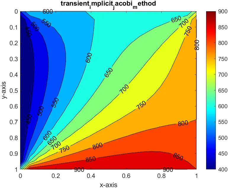
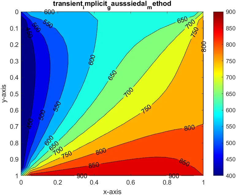
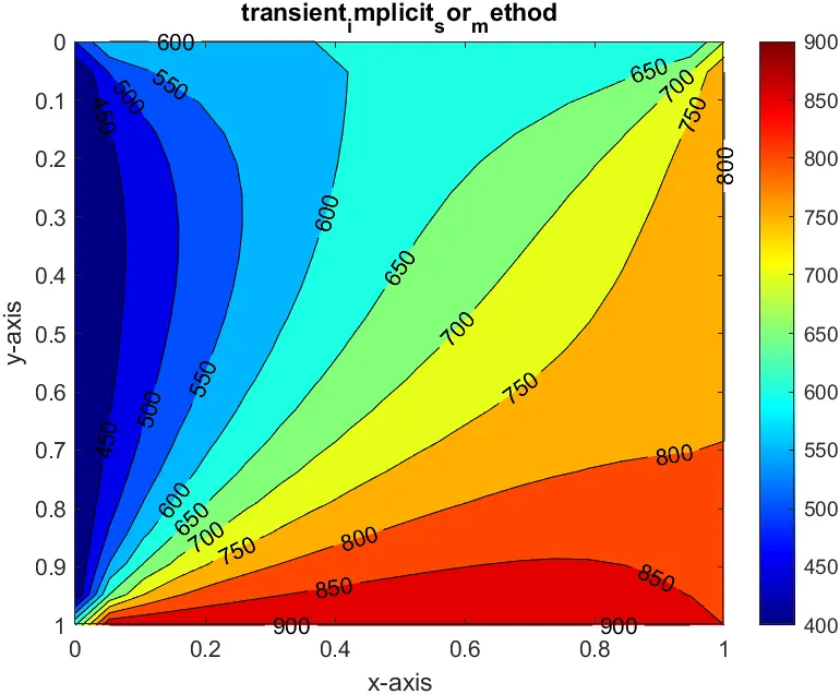
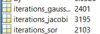
Conclusion: Here we can see that jacobi>gausssiedal>SOR,and in this problem we can understand that steady and unsteady heat conduction where steady means linear flow and unsteady means non-linear .

In steady state the temperature will be constant.

In unsteady(transient) the time required to change one state to another.

Explicit method ,is that direct method,without iterations we can solve .

Implicit methos,is that we are using iterations methods like(jacobi,gaussiedal,sor).