Week 5.1 - Mid term project - Solving the steady and unsteady 2D heat conduction problem
Aim :- To write down a MATLAB programming to solve 2 Dimensional Heat Conduction problem using both Steady and Transient state analysis.
Objectives :-
- Our main objective is to solve 2 d heat conduction equation using Implicit (Jacobi , Gauss seidel , Successive over relaxation) and Explicit (Direct) methods for steady and unsteady state analysis numerically
- Understand the governing equation of the Implicit and Explicit methods
- To compare the difference between the three types of iterative solvers in terms of convergence rate , time taken during solution
- And to plot the Temperature profile to observe the difference in result
Boundary conditions:-
Top Boundary = 600 K
Bottom Boundary = 900 K
Left Boundary = 400 K
Right Boundary = 800 K
Introduction :-
Steady state : If the variables of a system ( called state variables) are unchanging in time than the system or the process is called as Steady state. This means that partial derivatives of this propeties of the sytem is zero with respect to time.
Unsteady state : When the variable of interest changes over time of a system than it is called Unsteady state.
Explicit and Implicit : Numerical solution schemes are often referred to as being explicit or implicit. When a direct computation of the dependent variables can be made in terms of known quantities , the computation is said to be explicit. If we have one single unknown , we use explicit method also called as direct method.
| Explicit method | Implicit method |
|
|
|
2. Mathematically, if Y(t) is the current syatem state and Y(t+`Deltat`) is the state at the later time (`Deltat` is a small time step), then for an explicit method Y(t+`Deltat`) = F(Y(t)) |
2. Mathematically, if Y(t) is the current syatem state and Y(t+`Deltat`) is the state at the later time (`Deltat`is a small time step), then for implicit method Y(t+`Deltat`) = F(Y(t+`Deltat`))+G(Y(t)) |
|
3. When we have one unknown we mainly use explixit method to solve the equation. |
3. When the equation are nonlinear and the number of unknown variables is more , under this conditions implicitly formulated eqautions are almost solved using iteratove techniques. |
Different types of Iterative Solvers used in most of the Engineering problem :
We will implement the following methods in problem for solving implicit equations.
- Jacobi : IN this method, the 2D heat conduction equation solves using calculating the value of Temperature at inner nodes using several iterations, in which each value of temperature will be previously assigned temperature values at nodes.
- Gauss-seidel : In this method, the 2D heat conduction equation solves, we are calculating the value of temperatures at inner nodes using several iterations, in which every value of temperature will be updated successively with respect to the previous iteration
- Successive over-relaxation : In this method, the 2D heat conduction equation solves. We are calculating the value of temperatures at inner nodes using several iterations, in which every value of temperature will be updated successively with respect to the previous iteration. And also “Relaxation factor” multiplies to the algebraic equation to alter the path of the iteration.
Governing equation fot the Steady state case :-
Generalized Heat conduction through 3 dimensional coordinates is
`α*({ ∂^2 T}/{∂x^2} + {∂^2 T}/{∂y^2} + {∂^2 T}/{∂z^2} ) = {∂T}/{∂t}`
2 dimensional heat conduction equation for the steady state,
`(∂^2T)/(∂x^2) + (∂^2T)/(∂y^2) = 0`
Since this eliptical profile we have descritizzed each using Central differencing schems .
`( (T_(i-1,j) -2*(T)_(i,j)+T_(i+1,j) )/{Δx^2})^n + ((T_(i,j-1) -2*(T)_(i,j)+T_(i,j+1) )/(Δy^2) )^n=0`
This is our final equation for steady state case of Jacobi iterative method ,
`T(i,j) = (((Told(i-1,j)+Told(i+1,j))/(dx^2))+((Told(i,j+1)+Told(i,j-1))/(dy^2)))/k`
where k = `2((delx^2+dely^2)/(delx^2*dely^2))`
Equation for the Gauss seidel method
`T(i,j) = (((T(i-1,j)+Told(i+1,j))/(dx^2))+((Told(i,j+1)+T(i,j-1))/(dy^2)))/k`
Equation for the Successive over relaxation method
`T(i,j) = (Told(i,j)*(1-omega)) + (omega*(((T(i-1,j)+Told(i+1,j))/(dx^2))+((Told(i,j+1)+T(i,j-1))/(dy^2))))/k`
where omega `(omega)`= over relaxation factor
CODE TO SOLVE THE 2 D HEAT CONDUCTION EQUATION USING ITERATIVE SOLVERS FOR STEADY STATE CASE
clear all                    %Cleared all the existing variables in workspace
close all                    %Close all the figure windows
clc                          %Cleared the command window

% Geometric parameters of the domain

L = 1;                        %Length  of the domain
Nx = 10;                      %Number of nodes in x direction
Ny =10;                       %Number of nodes in y direction
x = linspace(0,1,Nx);
y = linspace(0,1,Ny);
dx = x(2) - x(1);             %Length of element along x direction
dy = y(2) - y(1);             %Length of element along y direction

% Boundary and Initial conditions
T_t = 600;
T_b = 900;
T_r = 800;
T_l = 400;

Ti = 300;                    %Initial temperature of the domain
T = Ti*ones(Nx,Ny);          %Temperature array
T(1,:) = 600;                %Assigning temperature for top wall
T(Nx,:) = 900;               %Assigning temperature for bottom wall
T(:,1) = 400;                %Assigning temperature for left wall
T(:,Ny) = 800;               %Assigning temperature for right wall

%Assigning temperature for the corners nodes
T(1,1) = 500;                %Assigning temperature for top-left corner
T(1,Ny) = 700;               %Assigning temperature for top-right corner
T(Nx,Ny) = 850;              %Assigning temperature for bottom-rigth corner
T(Nx,1) = 650;               %Assigning temperature for bottom-left corner


Told=T;

Error = 100;
tol = 1e-4;
k = 2*(dx^2+dy^2)/(dx^2*dy^2);

method = input('Iterative method = '); % For iterative method selection

%% JACOBI ITERATIVE METHOD

if (method==1)
    tic;
    jacobi_iter = 1;

    while(Error > tol)
        for i = 2:(Nx-1)
            for j = 2:(Ny-1)
                T(i,j) = (((Told(i-1,j)+Told(i+1,j))/(dx^2))+((Told(i,j+1)+Told(i,j-1))/(dy^2)))/k;
            end
        end

        Error = max(max(abs(T-Told)));     %Calculating the error
        Told = T;                          %Updating the old velocity
        jacobi_iter = jacobi_iter+1;
        time_taken = toc;

    end


    % Plotting for jacobi iterative method
    figure(1)
    contourf(x,y,T,'ShowText','on');
    colormap(jet);
    colorbar;
    xlabel('X')
    ylabel('Y')
    title_text  = sprintf('Iteration number = %d', jacobi_iter);
    title_text_1  = sprintf('Simulation time = %f', time_taken);
    title({'Steady state heat condustion profile by jacobi'; title_text;title_text_1});


end


%% GAUSS SIEDEL ITERATIVE METHOD

if (method==2)
    tic;
    gauss_iter = 1;

    while(Error > tol)
        for i = 2:(Nx-1)
            for j = 2:(Ny-1)
                T(i,j) = (((T(i-1,j)+Told(i+1,j))/(dx^2))+((Told(i,j+1)+T(i,j-1))/(dy^2)))/k;

            end
        end
        Error = max(max(abs(T-Told)));     %Calculating the error
        Told = T;                          %Updating the old velocity
        gauss_iter = gauss_iter+1;
        time_taken = toc;
    end

    % Plotting for gauss-siedel method
    figure(2)
    contourf(x,y,T,'ShowText','on');
    colormap(jet);
    colorbar;
    xlabel('X')
    ylabel('Y')
    title_text  = sprintf('Iteration number = %d', gauss_iter);
    title_text_1  = sprintf('Simulation time = %f', time_taken);
    title({'Steady state heat condustion profile by gauss siedel'; title_text;title_text_1})

end


%% SUCCESSIVE OVER RELAXATION ITERATIVE METHOD

if (method==3)
    tic;
    sor_iter = 1;
    omega = 1.4;                     %Over relaxation factor

    while(Error > tol)
        for i = 2:(Nx-1)
            for j = 2:(Ny-1)

                T(i,j) = (Told(i,j)*(1-omega)) + (omega*(((T(i-1,j)+Told(i+1,j))/(dx^2))+((Told(i,j+1)+T(i,j-1))/(dy^2))))/k;

            end
        end
        Error = max(max(abs(T-Told)));     %Calculating the error
        Told = T;                          %Updating the old velocity
        sor_iter = sor_iter+1;
        time_taken = toc;
    end

    % Plotting for sor method
    figure(3)
    contourf(x,y,T,'ShowText','on');
    colormap(jet);
    colorbar;
    xlabel('X')
    ylabel('Y')
    title_text  = sprintf('Iteration number = %d', sor_iter);
    title_text_1  = sprintf('Simulation time = %f', time_taken);
    title({'Steady state heat condustion profile by sor'; title_text;title_text_1});

end
Explanation of the code:-
- First of all as usual clear all, close all and clc has been used
- Then inputs for this problem has been assigned such as L(Length of the domain), number of nodes along x and y direction and initialization has been done for all the nodes.
- At next line we have created the x array and y array using linspace command and calculated the length of an element (dx, dy ) along x and y direction
- Next boundary condition of temperature for all the side of the domain and for all the four corners element has assigned
- As we wanted to write down the codes for all the four iterative methods in one single script file we have assigned iterative solver as input usinf if command
- Convergence loop has been created using for loop and it will iterate till the Error terms becomes less than tolerance. As it is 2 dimensional so 2 for loop has created inside the convergence loop and we are solving the equation for all the interior nodes in the domain.
- After the end of the convergence loop velocity has updated so that for the next iteration T will be the old temperature.
- At last, plotting has been done using suitable inbuilt command available in MATLAB.
Output:-
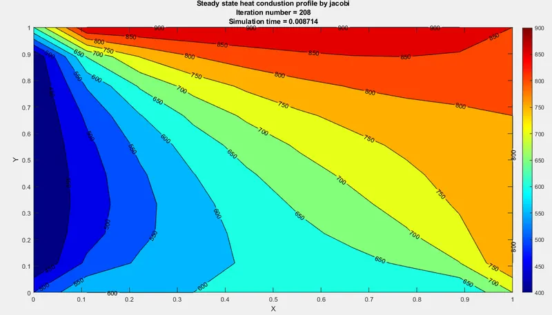
For Jacobi solver
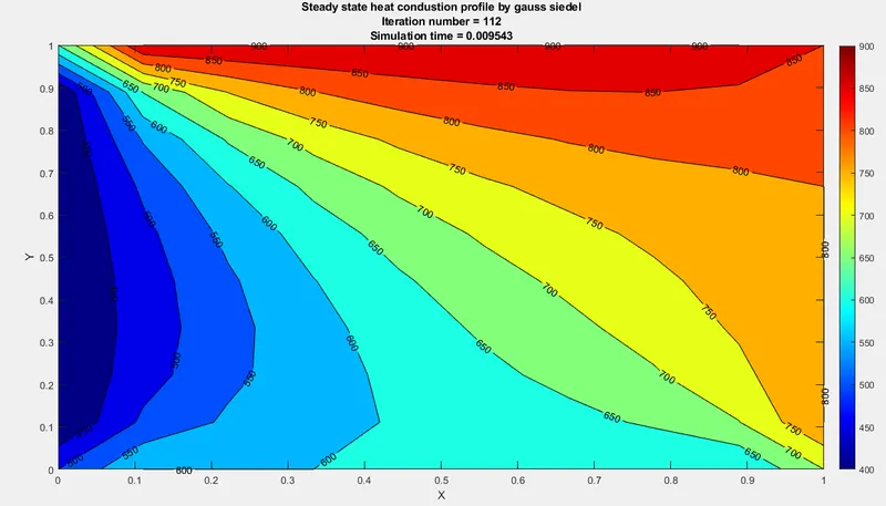
For Gauss siedel solver
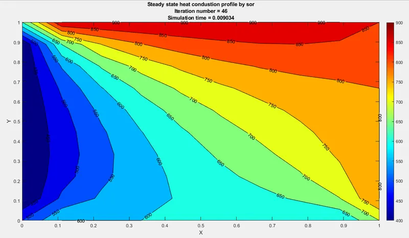
For Successive over relaxation solver
Observation:-
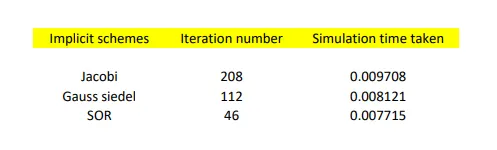
- In the above heat conduction equation for steady state case output, we can say that the no of iterations are vary for every method used.
- Jacobi method requires high no. of iterations as you can see in the above plot beacause this method uses same old values for entire calculations till it gets stable.
- Gauss Seidal method requires less no. of iterations for same given inputs as compare to Jacobi method because it uses updated values of T i.e. after calculating the value of T at certain node then it uses that updated value of T for next node.
- Successive over relaxation requires relatively very less no. of iterations compare to other cases to get stable, as it uses same equation as gauss seidal but it also uses Relaxation Factor ω which makes it to calculate faster. Also the relaxation factor affects the speed of calculation i.e if we use higher ω which will cause it to overshoot and make SOR slower causing it high no. of iterations.
Governing equation fot the Unsteady state case :-
Generalized Heat conduction equation for the unsteady state through 3 dimensional coordinates is
`α*({ ∂^2 T}/{∂x^2} + {∂^2 T}/{∂y^2} + {∂^2 T}/{∂z^2} ) = {∂T}/{∂t}`
By discretizing the second order term using central differencing and the temporal terms using first order differencing we get,
`α((T_(i-1,j) - 2*(T)_(i,j)+T_(i+1,j) )/{Δx^2} + (T_(i,j-1) - 2*(T)_(i,j)+T_(i,j+1) )/{Δy^2}) = {(T^(n+1))_(i,j) - (T^n)_(i,j)}/{Δt}`
And by simplifyinh this equation we have
`(T^(n+1))_(i,j) = ((T^n)_(i,j) + K_1(T^(n+1))_(i-1,j )+ K_1 (T^(n+1))_(i+1,j) + K_2(T^(n+1))_(i,j-1) + K_2(T^(n+1))_(i,j+1))/((1+ 2 K_1 + 2 K_2))`
where , K_1 = `K_1 =α {∆t}/{(Δx)^2}`
K_2 = `K_2 =α{∆t}/{(Δy)^2}`
`alpha`is the thermal diffusivity, measures the heat transfer from the hot material to the cold.
CODE TO SOLVE THE 2 D HEAT CONDUCTION EQUATION USING ITERATIVE SOLVERS FOR UNSTEADY STATE CASE
clear all                    %Cleared all the existing variables in workspace
close all                    %Close all the figure windows
clc                          %Cleared the command window

% Geometric parameters of the domain

L = 1;                        %Length  of the domain
Nx = 10;                      %Number of nodes in x direction
Ny =10;                       %Number of nodes in y direction
nt = 300;                     %Number of steps
x = linspace(0,1,Nx);
y = linspace(0,1,Ny);
dx = x(2) - x(1);             %Length of element along x direction
dy = y(2) - y(1);             %Length of element along y direction

% Boundary and Initial conditions
Ti = 300;                    %Initial temperature of the domain
T = Ti*ones(Nx,Ny);          %Temperature array
T(1,:) = 600;                %Assigning temperature for top wall
T(Nx,:) = 900;               %Assigning temperature for bottom wall
T(:,1) = 400;                %Assigning temperature for left wall
T(:,Ny) = 800;               %Assigning temperature for right wall

%Assigning temperature for the corners nodes
T(1,1) = 500;                %Assigning temperature for top-left corner
T(1,Ny) = 700;               %Assigning temperature for top-right corner
T(Nx,Ny) = 850;              %Assigning temperature for bottom-rigth corner
T(Nx,1) = 650;               %Assigning temperature for bottom-left corner

dt = 0.01; %time step
Told=T;
alpha = 0.3; % Thermal diffusivity
tprev_dt = Told;

tol = 1e-4;
k1 = alpha*dt/(dx^2);
k2 = alpha*dt/(dy^2);

method = input('Iterative method = '); %iterative method selection

%% JACOBI ITERATIVE METHOD

if (method==1)
    tic;
    jacobi = 1;
    for p = 1:nt
        error =100;
        while(error>tol)
            for i = 2:(Nx-1)
                for j = 2:(Ny-1)
                    term1 = (1+(2*k1)+(2*k2))^-1;
                    term2 = k1*term1;
                    term3 = k2*term1;
                    h = (Told(i-1,j)+Told(i+1,j));
                    v = (Told(i,j+1)+Told(i,j-1));
                    T(i,j) = ((tprev_dt(i,j)*term1)+(h*term2)+(v*term3));
                end
            end
            error = max(max(abs(T-Told)));
            Told = T;
            jacobi = jacobi+1;
        end
        tprev_dt = T ;
    end
    time_taken = toc;
    %plotting
    figure(1)
    contourf(x,y,T,'ShowText','on');
    colormap(jet);
    colorbar;
    xlabel('X')
    ylabel('Y')
    text1 = sprintf('number of iteration = %d', jacobi);
    text2 = sprintf('simulation time = %f', time_taken);
    title({'Transient state heat conduction profile Implicit-Jacobi'; text1; text2});
end


%% GAUSS-SEIDEL ITERATIVE METHOD

if (method==2)
    tic;
    gauss = 1;
    for p = 1:nt
        error =100;
        while(error>tol)
            for i = 2:(Nx-1)
                for j = 2:(Ny-1)
                    term1 = (1+(2*k1)+(2*k2))^-1;
                    term2 = k1*term1;
                    term3 = k2*term1;
                    h = (T(i-1,j)+Told(i+1,j));
                    v = (Told(i,j+1)+T(i,j-1));
                    T(i,j) = ((tprev_dt(i,j)*term1)+(h*term2)+(v*term3));
                end
            end

            error = max(max(abs(T-Told)));
            Told = T;
            gauss = gauss+1;
        end
        tprev_dt = T;
    end
    time_taken = toc;

    %plotting
    figure(1)
    contourf(x,y,T,'ShowText','on');
    colormap(jet);
    colorbar;
    xlabel('X')
    ylabel('Y')
    text1 = sprintf('number of iteration = %d', gauss);
    text2 = sprintf('simulation time = %f', time_taken);
    title({'Transient state heat conduction profile Implicit-Gauss-seidel'; text1; text2});
end

%% SUCCESSIVE OVER RELAXATION ITERATIVE METHOD

if (method==3)
    tic;
    sor = 1;
    omega = 1.2; % Over relaxation factor
    for p = 1:nt
        error =100;
        while(error>tol)

            for i = 2:(Nx-1)
                for j = 2:(Ny-1)

                    term1 = (1+(2*k1)+(2*k2))^-1;
                    term2 = k1*term1;
                    term3 = k2*term1;
                    h = (T(i-1,j)+Told(i+1,j));
                    v = (Told(i,j+1)+T(i,j-1));
                    T(i,j) = (Told(i,j)*(1-omega))+(omega*((tprev_dt(i,j)*term1)+(h*term2)+(v*term3)));
                end
            end

            error = max(max(abs(T-Told)));
            Told = T;
            sor = sor+1;
        end
        tprev_dt = T ;
    end
    time_taken = toc;

    %plotting
    figure(1)
    contourf(x,y,T,'ShowText','on');
    colormap(jet);
    colorbar;
    xlabel('X')
    ylabel('Y')
    text1 = sprintf('number of iteration = %d', sor);
    text2 = sprintf('simulation time = %f', time_taken);
    title({'Transient state heat conduction profile Implicit-SOR'; text1; text2});


end
Explanation :-
- First of all we have assigned the required inputs for thsi problem and then initialization and boundary condition for he each domain and the corners nodes has done.
- Then we have taken time step size dt as 0.01 and alpha , thermal diffusivity as 0.3 and we have given the iterative method as input so that we can calculate the all the three method in one single script file.
- Next created the space loop and convergence loop inside the space loop . The convergence loop will run till the errror value becomes small than tolerance.
- Indide the convergence loop two for loop ( because of the 2 dimensional domain) has created to solve the governing equation in each nodes along the x and y direction.
- Then we closed the two for loop and calculated the errror inside the convergence loop .
- Also updated the old velocity and the iteration number in order to visualize the iteration number in output.
- Thus space loop come to an end.
Output:-
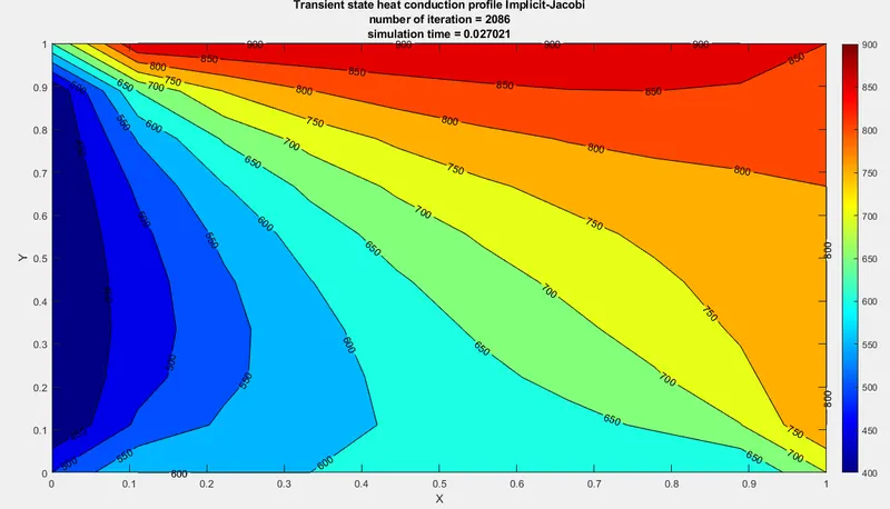
For Jacobi solver
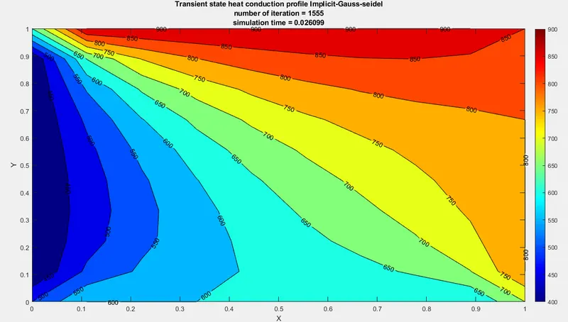
For Gauss siedel solver
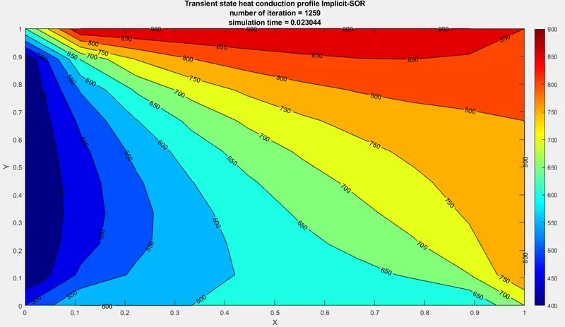
For successive over relaxation solver
Observation:-
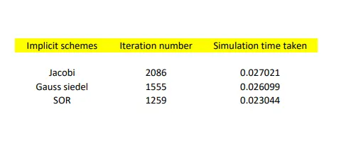
- In the above heat conduction equation for steady state case output, we can say that the no of iterations are vary for every method used.
- Jacobi method requires high no. of iterations as you can see in the above plot beacause this method uses same old values for entire calculations till it gets stable.
- Gauss Seidal method requires less no. of iterations for same given inputs as compare to Jacobi method for same number of dt and nt because it uses updated values of T i.e. after calculating the value of T at certain node then it uses that updated value of T for next node.
- Successive over relaxation requires relatively very less no. of iterations compare to other cases to get stable, as it uses same equation as gauss seidal but it also uses Relaxation Factor ω which makes it to calculate faster. Also the relaxation factor affects the speed of calculation i.e if we use higher ω which will cause it to overshoot and make SOR slower causing it high no. of iterations.
Explicit Method for Transient case:-
When we have pnly one unknowns we use Explicit chemes. And for exlicit , we need to use iterative methods as we have only one unknowns.
`T^(n+1)(i,j) = T^n(i,j) + k1(T(i+1,j) - 2T(i,j) + T(i-1,j))^n + k2(T(i,j+1) - 2T(i,j) + T(i,j-1)) ^n`
MATLAB CODE TO SOLVE UNSTEADY HEAT CONDUCTION EQUATION USING EXPLICIT SCHEME
clear all                    %Cleared all the existing variables in workspace
close all                    %Close all the figure windows
clc                          %Cleared the command window

% Geometric parameters of the domain

L = 1;                        %Length  of the domain
Nx = 10;                      %Number of nodes in x direction
Ny =10;                       %Number of nodes in y direction
nt = 300;                     %Number of steps
x = linspace(0,1,Nx);
y = linspace(0,1,Ny);
dx = x(2) - x(1);             %Length of element along x direction
dy = y(2) - y(1);             %Length of element along y direction

% Boundary and Initial conditions
Ti = 300;                    %Initial temperature of the domain
T = Ti*ones(Nx,Ny);          %Temperature array
T(1,:) = 600;                %Assigning temperature for top wall
T(Nx,:) = 900;               %Assigning temperature for bottom wall
T(:,1) = 400;                %Assigning temperature for left wall
T(:,Ny) = 800;               %Assigning temperature for right wall

%Assigning temperature for the corners nodes
T(1,1) = 500;                %Assigning temperature for top-left corner
T(1,Ny) = 700;               %Assigning temperature for top-right corner
T(Nx,Ny) = 850;              %Assigning temperature for bottom-rigth corner
T(Nx,1) = 650;               %Assigning temperature for bottom-left corner

dt = 0.01; %time step
Told=T;
alpha = 0.3; % Thermal diffusivity

k1 = (alpha*dt)/(dx^2);
k2 = (alpha*dt)/(dy^2);
CFL = (alpha*dt)/(dx^2);

%EXPLICIT METHOD
% running for loop

tic;
explicit = 1;
for p = 1:nt
    for i = 2:(Nx-1)
        for j = 2:(Ny-1)
            term1 = (Told(i-1,j)-2*Told(i,j)+Told(i+1,j));
            term2 = (Told(i,j-1)-2*Told(i,j)+Told(i,j+1));
            T(i,j) = ((Told(i,j))+(k1*term1)+(k2*term2));
        end
    end

    Told = T;
    explicit = explicit+1;
end

time_taken = toc;

%Plotting
figure(1)
contourf(x,y,T,'ShowText','on');
colormap(jet);
colorbar;
xlabel('X')
ylabel('Y')
text1 = sprintf('Iteration number = %d', explicit );
text2 = sprintf('simulation time = %f', time_taken);
title({'Transient state heat conduction'; text1; text2});
Output:
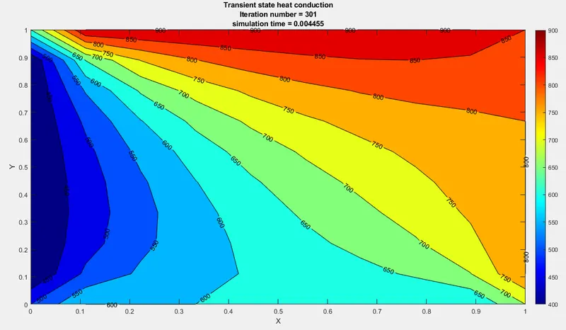
Explanation:- Here as we using explicit method, so we need to make sure that CFL or Courant number should be <= 0.5 to make the solution stable. Here CFL = k1 + k2. In our case after assuming nt = 300 and dt = 0.01 , we get CFL number is 0.2430 . So, solution is stable.
Conclusion :-
- By observing all of the outputs for steady and unsteady state cases it can be said that steady state equation requires less number of iterations and less simulation time than unsteady state equation.
- Successive over relaxation method becomes stable and gives solution in lesser time compare to other two iterative methods in both steady and unsteady state cases.
- Also for the same number of nt and dt value explicit schemes takes less time compare to implicit schemes.
- And CFL number should be less than or eqaul 0.5 for explicit method to become the solution stable.
References :-
https://skill-lync.com/knowledgebase/courant-number
L.Pareschi, G.Russo: Implicit-Explicit Runge-Kutta schemes for stiff systems of differential equations, Recent Trends in Numerical Analysis, Vol. 3, 269-289, 2000