AIM:
To solve the 2d heat conduction equation Steady state analysis & Transient State Analysis by using the point iteration technique.
- Jacobi
- Gauss sediel
- Successive over relaxation
Transient state analysis using explicit and implicit schemes.
Given
- Absolute error criteria is 1e-4
- Domain is a unit square, length L = 1 m
- Number of points along the x direction is equal to the number of points along the y direction, 'nx = ny'.
Boundary Temperatures
- Top Boundary = 600 K
- Bottom Boundary = 900 K
- Left Boundary = 400 K
- Right Boundary = 800 K
2D Heat Conduction equation:
`(delT)/(delt) = alpha( (del^2T)/(delx^2)+(del^2T)/(dely^2))`
1. Steady state solution:
`( (del^2T)/(delx^2)+(del^2T)/(dely^2)) = 0`
Descretizing the Steady state condition
`(T_(i-1,j) - 2T_(i,j)+ T_(i+1,j))/(Deltax^2) + (T_(i,j+1) - 2T_(i,j)+ T_(i,j-1))/(Deltay^2) = 0`
`T_(i,j) = 1/k (T_(i-1,j) + T_(i+1,j))/(Deltax^2) + (T_(i,j+1) + T_(i,j-1))/(Deltay^2)`
where
`k = (Deltax^2 + Delta y^2)/(Deltax^2 . Delta y^2)`
The above equation is solving by using Iterative solvers, Jacobi, Gauss sediel, SOR.The above equation gives the Temperature values at each node of its neighboring nodes.
Jacobi Method:
`T_(i,j)^(n+1) = 1/k ((T_(i-1,j)^n+T_(i+1,j)^n)/(Deltax^2) + (T_(i,j-1)^n+T_(i,j+1)^n)/(Deltay^2))`
In Jacobi method ,`T^(n+1)`iteration is calculated with previous value 'T' at nth `iteration untill the solution converge
Gauss seidal Method:
`T_(i,j)^(n+1) = 1/k ((T_(i-1,j)^(n+1)+T_(i+1,j)^n)/(Deltax^2) + (T_(i,j-1)^(n+1)+T_(i,j+1)^n)/(Deltay^2))`
In gauss seidal method the value of `T^(n+1)`iteration are calculated with (n+1) iteration which is already computed
Succive over relaxation:
`T_(i,j)^(n+1) = T_(i,j)^n (1-alpha) + alpha/k . T_(GS) or Jacobi`
SOR is a fast converge method ,it is a advance versionn of gauss sedial method for solving linear system of equations. sor uses the result of gauss and scale the convegence by relaxation factor (Omega)
Matlab coding for steady state:
close all
clear all
clc
nx = 20; %nx & ny are nodes along the length of x & y respectively
ny = nx;
x = linspace(0,1,nx);
y = linspace(0,1,ny);
dx=(x(2)-x(1));
dy=(y(2)-y(1));
k=2* (dx^2 + dy^2)/(dx^2 * dy^2);
% Boundary conditions
top=600;
bottom=300;
left=400;
right=800;
% Taking all values as ones - nx rows and ny columns
T = ones(nx,ny);
% Assiging those boundary conditions to the T matrix excepting the corners
T(1,2:nx-1) = top;
T(ny,2:nx-1) = bottom;
T(2:ny-1,1) = left;
T(2:ny-1,nx) = right;
% Assigning the values at the corner positions of the T matrix by taking average of adjacent values
T(1,1)=(top+left)/2;
T(ny,1)=(bottom+left)/2;
T(1,nx)=(right+top)/2;
T(ny,nx)=(right+bottom)/2;
% T variables are created for updating the values
Told=T;
Told1=T;
Told2=T;
Told3=T;
Told4=T;
% Assigining the error value for each method
error_jacobi =1;
error_gauss = 1;
error_SOR = 1;
tolerance = 1e-4;
% Start Every iteration with '1'
jacobi_iteration=1;
Gauss_iteration=1;
SOR_iteration=1;
%for SOR method
alpha=1.5; %alpha should be between 0 & 2
% Jacobi Method
tic
while (error_jacobi > tolerance)
for i = 2:nx-1 %space loop
for j = 2:ny-1
T(i,j) = 1/k * ((Told(i+1,j)+Told(i-1,j))/dx^2+(Told(i,j+1)+Told(i,j-1))/dy^2);
end
end
error_jacobi = max(max(abs(Told-T)));
Told = T;
jacobi_iteration = 1+jacobi_iteration;
end
a=toc;
fprintf('Computational time using Jacobi method = %g n',a);
fprintf('No. of iterations in Jacobi method = %d n',jacobi_iteration);
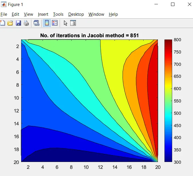
figure(1)
contourf(T); % To get output as contour
colormap(jet); % Color of contour to get rainbow colors
colorbar; % Side bar representing the temperature with color
title_text = sprintf('No. of iterations in Jacobi method = %d',jacobi_iteration);
title(title_text);
set(gca, 'YDir','reverse')
% Gauss-Seidel Method
tic
while (error_gauss > tolerance)
for i = 2:nx-1
for j = 2:ny-1
Told1(i,j) = ((Told1(i+1,j)+Told1(i-1,j))/dx^2+(Told1(i,j+1)+Told1(i,j-1))/dy^2)/k;
end
end
error_gauss = max(max(abs(Told2-Told1)));
Told2 = Told1;
Gauss_iteration = Gauss_iteration+1;
end
b=toc;
fprintf(' nComputational time using Gauss-seidel method = %g n',b);
fprintf('No. of iterations in Gauss-seidel method = %d n',Gauss_iteration);
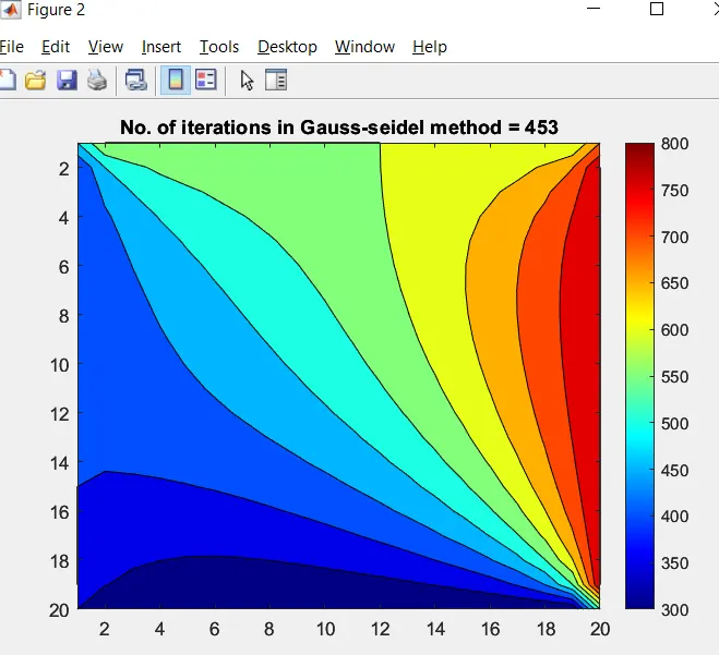
figure(2)
contourf(Told1);
colormap(jet);
colorbar;
title_text = sprintf('No. of iterations in Gauss-seidel method = %d',Gauss_iteration);
title(title_text);
set(gca, 'YDir','reverse')
% Successive over-relaxation (SOR) Method
tic
while (error_SOR > tolerance)
for i = 2:nx-1
for j = 2:ny-1
Told3(i,j) = (1-alpha)*Told4(i,j)+(alpha/k)*((Told3(i+1,j)+Told3(i-1,j))/dx^2+(Told3(i,j+1)+Told3(i,j-1))/dy^2);
end
end
error_SOR = max(max(abs(Told4-Told3)));
Told4 = Told3;
SOR_iteration = SOR_iteration+1 ;
end
c=toc;
fprintf(' nComputational time using SOR method = %g n',c);
fprintf('No. of iterations in SOR method = %d n',SOR_iteration);
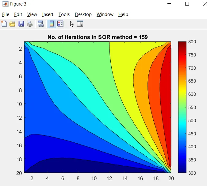
figure(3)
contourf(Told3);
colormap(jet);
colorbar;
title_text = sprintf('No. of iterations in SOR method = %d',SOR_iteration);
title(title_text);
set(gca, 'YDir','reverse')
Graphs for steady state:
Result:
As comparing above plots the SOR is converge with less iteratives as comapare to gauss & jacobi.
1.2 Transient State analysis:
1.2.1 Solving Implicit
`(T_(i-1,)^(n+1) - T_(i,j)^(n)) / (Delta t) = alpha(( T_(i-1,j)-2T_(i,j)+T_(i+1,j ))/(Delta x^2)+ (T_ (i,j-1)-2T_(i,j)+T_(i,j+1))/(Deltay^2))^(n+1)`
Consider
`k_1 = alpha (Delta t)/ (Delta x^2) and k_2 = alpha (Delta t)/ (Delta y^2)`
simplifing the above equation
`T_(i,j)^(n+1) .(1+2k_1+2k_2) = T_(i,j)^n + k_1(T_(i-1,j)+T_(i+1,j))^(n+1) + k_2(T_(i,j-1)+T_(i,j+1))^(n+1)`
`T_(i,j)^(n+1) =( T_(i,j)^n + k_1(T_(i-1,j)+T_(i+1,j))^(n+1) + k_2(T_(i,j-1)+T_(i,j+1))^(n+1))/(1+2k_1+2k_2)`
Consider
term 1 = `1/(1+2k_1+2k_2)`
term2 = `k_1 .term1`
term3 =`k_3.term1`
`T_(i,j)^(n+1)= term1.T_(i,j)^n + term2.(T_(i-1,j)+T_(i+1,j))^(n+1) + term3.(T_(i,j-1)+T_(i,j+1))^(n+1)`
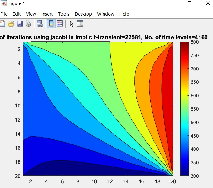
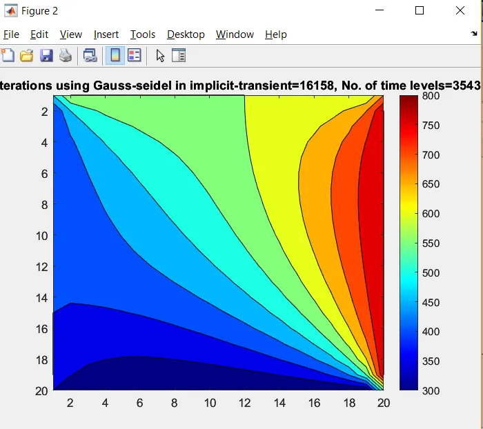
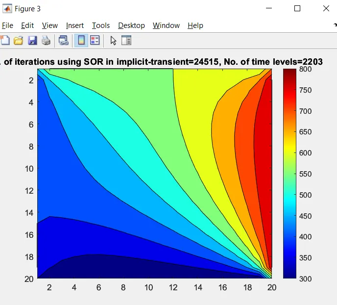
Matlab coding for Transient Implicit :
close all
clear all
clc
nx = 20;
ny = nx;
x = linspace(0,1,nx);
y = linspace(0,1,ny);
dx=(x(2)-x(1));
dy=(y(2)-y(1));
thermal_diffusity = 1.4;
dt = 4e-4;
time=5;
k1 = thermal_diffusity*dt/dx^2;
k2 = thermal_diffusity*dt/dy^2;
nt = time/dt;
% Boundary conditions
top=600;
bottom=300;
left=400;
right=800;
% Taking all values as ones - nx rows and ny columns
T = ones(nx,ny);
% Boundary conditions to the T matrix excepting the corners
T(1,2:nx-1) = top;
T(ny,2:nx-1) = bottom;
T(2:ny-1,1) = left;
T(2:ny-1,nx) = right;
% Assigning the values at the corner positions of the T matrix by taking average of adjacent values
T(1,1)=(top+left)/2;
T(ny,1)=(bottom+left)/2;
T(1,nx)=(right+top)/2;
T(ny,nx)=(right+bottom)/2;
term1 = 1/(1+2*k1+2*k2);
term2 = k1* term1;
term3 = k2* term1;
% Dummy variables are created for updating the values of next time step
Tprev1=T; %for jacobi
Tprev2=T; %for Gauss-seidel
Tprev3=T; %for SOR
% variables are created for updating the values
Told=T;
Told1=T;
Told2=T;
Told3=T;
Told4=T;
tolerance = 1e-7;
% start with iteration number 1
j_iteration=1;
GS_iteration=1;
SOR_iteration=1;
% all method should be started with 1st time loop
j_time=1;
GS_time=1;
SOR_time=1;
%for SOR method
alpha=1.5; %alpha should be between 1 & 2
k=2* (dx^2 + dy^2)/(dx^2 * dy^2);
%jacobi method - transient state - implicit scheme
tic
for t=1:nt %time loop
error_jacobi = 9e9;
while (error_jacobi > tolerance)
for i = 2:nx-1 %space loop
for j = 2:ny-1
H1 = Told(i+1,j)+Told(i-1,j);
V1 = Told(i,j+1)+Told(i,j-1);
T(i,j) = (term1*Tprev1(i,j))+(term2*H1)+(term3*V1);
end
end
error_jacobi= max(max(abs(Told-T)));
Told= T;
j_iteration = 1+j_iteration;
end
Tprev1=T;
j_time=1+j_time;
if (error_jacobi==0)
break
end
end
a=toc;
fprintf('n Computational time using implicit Jacobi method = %g n',a);
fprintf('No. of iterations in implicit Jacobi method = %d n',j_iteration);
fprintf('No. of time levels approached in implicit Jacobi method = %d n',j_time);
figure(1)
contourf(T);
colormap(jet);
colorbar;
title_text = sprintf('No. of iterations using jacobi in implicit-transient=%d, No. of time levels=%g',j_iteration,j_time);
title(title_text) %title of plot
set(gca, 'YDir','reverse')
% Gauss_seidel method - transient state - implicit scheme
tic
for t=1:nt %time loop
error_gauss = 9e9;
while (error_gauss > tolerance)
for i = 2:nx-1 %space loop
for j = 2:ny-1
H2 = Told2(i+1,j)+Told1(i-1,j);
V2 = Told2(i,j+1)+Told1(i,j-1);
Told1(i,j) = (term1*Tprev2(i,j))+(term2*H2)+(term3*V2);
end
end
error_gauss= max(max(abs(Told2-Told1)));
Told2= Told1;
GS_iteration = 1+GS_iteration;
end
Tprev2=Told2;
GS_time=1+GS_time;
if (error_gauss==0)
break
end
end
b=toc;
fprintf('n Computational time using implicit GS method = %g n',b);
fprintf('No.of iterations in implicit GS method = %d n',GS_iteration);
fprintf('No.of time levels approached in implicit GS method = %d n',GS_time);
figure(2)
contourf(Told1);
colormap(jet);
colorbar;
title_text = sprintf('No. of iterations using Gauss-seidel in implicit-transient=%d, No. of time levels=%g',GS_iteration,GS_time);
title(title_text) %title of plot
set(gca, 'YDir','reverse')
% SOR method - transient state - implicit scheme
tic
for t=1:nt %time loop
error_SOR = 9e9;
while (error_SOR > tolerance)
for i = 2:nx-1 %space loop
for j = 2:ny-1
H3 = Told4(i+1,j)+Told3(i-1,j);
V3 = Told4(i,j+1)+Told3(i,j-1);
Told3(i,j) = (1-alpha)*Told4(i,j)+(alpha)*((term1*Tprev3(i,j))+(term2*H3)+(term3*V3));
end
end
error_SOR= max(max(abs(Told4-Told3)));
Told4=Told3;
SOR_iteration = 1+SOR_iteration;
end
Tprev3=Told4;
SOR_time=1+SOR_time;
if (error_SOR<1e-10)
break
end
end
c=toc;
fprintf('n Computational time using implicit SOR method = %g n',c);
fprintf('No. of iterations in implicit SOR method = %d n',SOR_iteration);
fprintf('No. of time levels approached in implicit SOR method = %d n',SOR_time);
figure(3)
contourf(Told3);
colormap(jet);
colorbar;
title_text = sprintf('No. of iterations using SOR in implicit-transient=%d, No. of time levels=%g',SOR_iteration,SOR_time);
title(title_text)
set(gca, 'YDir','reverse')
Plots:
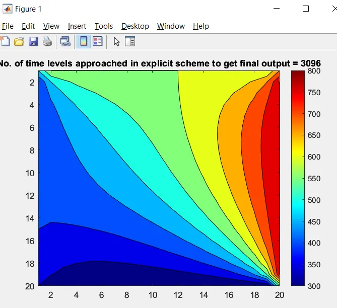
1.2.2 Solving Explicit:
Explicit scheme solve directly without any resulting in system of linear equations, eplicit scheme does not required iteration solver.
`(delT)/(delt)=alpha ( (del^2T)/(delx^2)+(del^2T)/(dely^2))`
`(T_(i-1,)^(n+1) - T_(i,j)^(n)) / (Delta t) = alpha(( T_(i-1,j)-2T_(i,j)+T_(i+1,j ))/(Delta x^2)+ (T_ (i,j-1)-2T_(i,j)+T_(i,j+1))/(Deltay^2))^(n)`
`k_1 = alpha (Delta t)/ (Delta x^2) and k_2 = alpha (Delta t)/ (Delta y^2)`
simplifying above equation:
`T_(i,j)^(n+1) = T_(i,j)^n .(1+2k_1+2k_2)+ k_1(T_(i-1,j)+T_(i+1,j))^n + k_2(T_(i,j-1)+T_(i,j+1))^n`
for stability`CFL <= 0.5`
`k_1=CFL_x & k_2 = CFL_y`
`CFL_x + CFL_y <= 0.5`
Matlab coding for Explicit:
close all
clear all
clc
nx = 20;
ny = nx;
x = linspace(0,1,nx);
y = linspace(0,1,ny);
dx=(x(2)-x(1));
dy=(y(2)-y(1));
thermal_diffusivity = 1.4;
dt = 4e-4;
time=5;
cfl = 2*thermal_diffusivity*(dt/dx^2);
k1 = thermal_diffusivity*dt/dx^2;
k2 = thermal_diffusivity*dt/dy^2;
nt = time/dt;
% Boundary conditions
top=600;
bottom=300;
left=400;
right=800;
% Taking all values as ones - nx rows and ny columns
Tfirst = ones(nx,ny);
% Boundary conditions for T matrix excepting the corners
Tfirst(1,2:nx-1) = top; % first row of T matrix
Tfirst(ny,2:nx-1) = bottom; % last row of T matrix
Tfirst(2:ny-1,1) = left; % first column of T matrix
Tfirst(2:ny-1,nx) = right; % last column of T matrix
% Corner positions to the T matrix by taking average of adjacent values
Tfirst(1,1)=(top+left)/2;
Tfirst(ny,1)=(bottom+left)/2;
Tfirst(1,nx)=(right+top)/2;
Tfirst(ny,nx)=(right+bottom)/2;
% variables are created for updating the values
Tprevious = Tfirst;
Tnew = Tfirst;
% starting with iteration number 1 for every method
plane_iter = 1;
term1 = (1-(2*k1)-(2*k2));
tolerance=1e-7;
%Transient state - explicit scheme
tic
for t=1:nt
error = 9e9;
for i = 2:nx-1
for j = 2:ny-1
H1=k1*(Tprevious(i+1,j)+Tprevious(i-1,j));
V1=k2*(Tprevious(i,j+1)+Tprevious(i,j-1));
Tnew(i,j) = (term1*Tprevious(i,j))+(H1)+(V1);
end
end
error = max(max(abs(Tprevious-Tnew)));
Tprevious = Tnew;
plane_iter = 1+plane_iter;
if error==0 % To stop the loop after reaching convergence
break
end
end
a=toc;
fprintf(' n Computational time using Explicit method = %g n',a);
fprintf(' No. of time levels approached in explicit method = %d n',plane_iter);
figure(1)
contourf(Tnew);
colormap(jet);
colorbar;
title_text = sprintf('No. of time levels approached in explicit scheme to get final output = %g',plane_iter );
title(title_text)
set(gca, 'YDir','reverse')
Graphs: