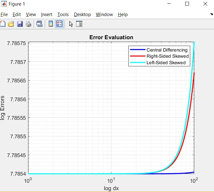
Week 3.5 - Deriving 4th order approximation of a 2nd order derivative using Taylor Table method

Aim: Derive the following fourth order approximation of the second order derivative

1. Central difference
2. Skewed right-sided difference
3. Skewed left-sided difference

To write a program in matlab to evaluate 2-order derivative of the analytical function 'exp(x)*cos(x)', and compare it with the 3 numerical approximations that have derived.

Taylor series

Taylor series of a function is the sum of infinite series or infinite terms.

`e^x = 1+x+(x^2)/(2!)+(x^3)/(3!)+(x^4)/(4!)+(x^5)/(5!)+....`

Deriving the fourth order approximations of a second order derivative Central difference

The number of nodes required for 4th order approximation of a Second order derivative can be given by the equation

N = P+Q-1

N is the number of nodes

p is the order of approximation

N = 2+4-1=5

The second order derivative with 4th order approximation

Hypothesis equation

`grad^2x f''(x)= af(i-2)+bf(i-1)+cf(i)+df(i+1)+ef(i+2)`--------(1)`

By using taylor seris evaluating hypothesis equation

`af(i−2) = a[f(i)−(2gradx)/(1!)f'(i)+(2gradx)^2/(2!)f''(i)−(2gradx)^3/(3!)f'''(i)+(2gradx)^4/(4!)−.........`

`bf(i−1) = b[f(i)−(gradx)/(1!)f'(i)+(gradx)^2/(2!)f''(i)−(gradx)^3/(3!)f'''(i)+(gradx)^4/(4!)−.........`

`cf(i)=cf(i)`

`df(i+1) = d[f(i)+(gradx)/(1!)f'(i)+(gradx)^2/(2!)f''(i)+(gradx)^3/(3!)f'''(i)+(gradx)^4/(4!)........`

`ef(i+2) = e[f(i)+(2gradx)/(1!)f'(i)+(2gradx)^2/(2!)f''(i)+(2gradx)^3/(3!)f'''(i)+(2gradx)^4/(4!).........`

Tailor table for Central difference

Taylor Table

Tailor seris expansion

Numerical stencil f(i) gradx f'(i) gradx^2 f'(i) gradx^3 f'''(i) gradx^4 f''''(i)

`gradx^2(del^2f)/(delx^2) f(i) gradxf'(i) gradx^2 f''(i) gradx^3 f'''(i) gradx^4 f''''(i)`

af(i-2) a -2a 4a/2 -8a/6 16a/24

bf(i-1) b -b b/2 -b/6 b/24

cf(i) c 0 0 0 0

df(i+1) d d d/2 d/6 d/24

ef(i+2) e 2e 4e/2 8e/6 16e/24

Evaluation for

2nd order 0 0 1 0 0

derivative

Now the equations to slove

a+b+c+d+e = 0

-2a – b + d + 2e =0

4a/2 + b/2 + d/2 + 4e/2 =1

-8a/6 - b/6 + d/6 + 8e/6 = 0

16a/24 + b/24 + d/24 + 16e/24 = 0

Converting the above equations into matrix form

`[[1,1,1,1,],[-2,-1,0,1,2],[4/2,1/2,0,1/2,4/2],[-8/6,-1/6,0,1/6,8/6],[16/24,1/24,0,1/24,16/24]]*[[a],[b],[c],[d],[e]]=[[0],[0],[1],[0],[0]]`

Solving the above matrices using MATLAB to find the values of the coefficient

A=[1,1,1,1,1;-2,-1,0,1,2;4/2,1/2,0,1/2,4/2;-8/6,-1/6,0,1/6,8/6;16/24,1/24,0,1/24,16/24;]

B=[0;0;1;0;0]

sol = inv(A) * B

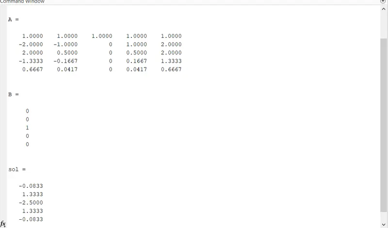
a= -0.0833, b= 1.3333, c= -2.5000, d= 1.3333, e= -0.0833

here a = e and b = d

Deriving the fourth order approximations of a second order derivative using skewed right side

The number of nodes required for 4th order approximation of a Second order derivative can be given by the equation

N = P+Q

N is the number of nodes

p is the order of approximation

N = 2+4=6

Hypothesis equation

`grad^2x f''(x)= af(i)+bf(i+1)+cf(i+2)+df(i+3)+ef(i+4)+gf(i+5)`-------(2)

By using taylor seris evaluating hypothesis equation

`af(i)=af(i)`

`bf(i+1)=b[f(i)+(gradx)/(1!)f'(i)+(gradx)^2/(2!)f''(i)+(gradx)^3/(3!)f'''(i)+(gradx)^4/(4!)f''''...`

`cf(i+1)=c[f(i)+(2gradx)/(1!)f'(i)+(2gradx)^2/(2!)f''(i)+(2gradx)^3/(3!)f'''(i)+(2gradx)^4/(4!)f''''...`

`df(i+3)=d[f(i)+(3gradx)/(1!)f'(i)+(3gradx)^2/(2!)f''(i)+(3gradx)^3/(3!)f'''(i)+(3gradx)^4/(4!)f''''...`

`ef(i+4)=e[f(i)+(4gradx)/(1!)f'(i)+(4gradx)^2/(2!)f''(i)+(4gradx)^3/(3!)f'''(i)+(4gradx)^4/(4!)f''''...`

`gf(i+5)=g[f(i)+(gradx)/(1!)f'(i)+(5gradx)^2/(2!)f''(i)+(5gradx)^3/(3!)f'''(i)+(5gradx)^4/(4!)f''''...`

Tailor table for skewed right side

Taylor Table

Tailor seris expansion

`gradx^2(del^2f)/(delx^2) f(i) gradxf'(i) gradx^2 f''(i) gradx^3 f'''(i) gradx^4 f''''(i) gradx^5 fiv(i)`

af(i-5) a -5a 25a/2 -125a/6 625a/24 -3125a/120

bf(i-4) b -4b 16b/2 -64b/6 256b/24 -1024b/120

cf(i-3) c -3c 9c/2 -27c/6 81c/24 -243c /120

df(i-2) d -2d 4d/2 -8d/6 16d/24 -32d/120

ef(i-1) e -e e/2 -e/6 e/24 -e/120

gf(i) g 0 0 0 0 0

Evaluation for

2nd order 0 0 1 0 0 0

derivative

Now the equations to slove

a+b+c+d+e+g = 0

b+2c+3d+4e+5g=0

b/2+4c/2+9d/2+16e/2+25g/2=1

b/6+8c/6+27d/6+64e/6+125g/6=0

b/24+16c/24+81d/24+256e/24+625g/24=0

b/120+32c/120+243d/120+1024e/120+3125g/120=0

Converting the above equations into matrix form

`[[1,1,1,1,1,1],[0,1,2,3,4,5],[0,1/2,4/2,9/2,16/2,25/2],[0,1/6,8/6,27/6,64/6,125/6],[0,1/24,16/24,81/24,256/24,625/24],[0,1/120,32/120,243/120,1024/120,3125/120]]*[[a],[b],[c],[d],[e],[g]]=[[0],[0],[1],[0],[0],[0]]`

Solving the above matrices using MATLAB to find the values of the coefficient

A=[1,1,1,1,1,1;0,1,2,3,4,5;0,1/2,4/2,9/2,16/2,25/2;0,1/6,8/6,27/6,64/6,125/6;0,1/24,16/24,81/24,256/24,625/24;0,1/120,32/120,243/120,1024/120,3125/120;]

B=[0;0;1;0;0;0]

sol = inv(A)* B

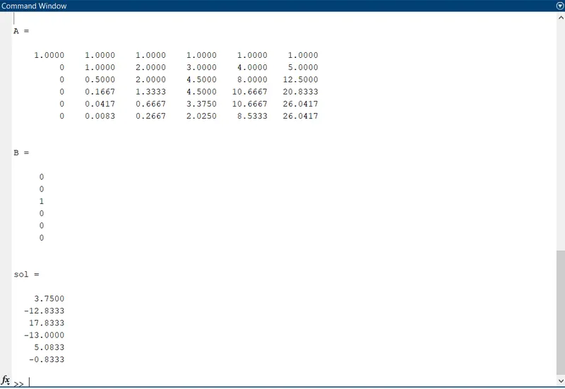
a=3.7500, b=-12.8333, c=17.8333, d=-13.0, e=5.0833, g=-0.8333

Deriving the fourth order approximations of a second order derivative using skewed left side

The number of nodes required for 4th order approximation of a Second order derivative can be given by the equation

N = P+Q

N is the number of nodes

p is the order of approximation

N = 2+4=6

Hypothesis equation

`grad^2x f''(x)= af(i-5)+bf(i-4)+cf(i-3)+df(i-2)+ef(i-1)+gf(i)`------(3)

By using taylor seris evaluating hypothesis equation

`af(i-5)=a[f(i)-(5gradx)/(1!)f'(i)+(5gradx)^2/(2!)f''(i)-(5gradx)^3/(3!)f'''(i)+(5gradx)^4/(4!)f''''...`

`bf(i-4)=b[f(i)-(4gradx)/(1!)f'(i)+(4gradx)^2/(2!)f''(i)-(4gradx)^3/(3!)f'''(i)+(4gradx)^4/(4!)f''''...`

`cf(i-3)=c[f(i)-(3gradx)/(1!)f'(i)+(3gradx)^2/(2!)f''(i)-(3gradx)^3/(3!)f'''(i)+(3gradx)^4/(4!)f''''...`

`df(i-2)=d[f(i)-(2gradx)/(1!)f'(i)+(2gradx)^2/(2!)f''(i)-(2gradx)^3/(3!)f'''(i)+(2gradx)^4/(4!)f''''...`

`ef(i-5)=e[f(i)-(gradx)/(1!)f'(i)+(gradx)^2/(2!)f''(i)-(gradx)^3/(3!)f'''(i)+(gradx)^4/(4!)f''''...`

`gf(i)=gf(i)`

Tailor table for skewed left side

Taylor Table

Tailor seris expansion

`gradx^2(del^2f)/(delx^2) f(i) gradxf'(i) gradx^2 f''(i) gradx^3 f'''(i) gradx^4 f''''(i) gradx^5 fiv(i)`

af(i) g 0 0 0 0 0

bf(i-1) b -b b/2 -b/6 b/24 -b/120

cf(i-2) c -2c 4c/2 -8c/6 16c/24 -32c/120

df(i-3) d -3d 9d/2 -27d/6 81d/24 -243d/120

ef(i-4) e -4e 16e/2 -64e/6 256e/24 -1024e/120

gf(i-5) g -5g 25g/2 -125g/6 625g/24 -3125g/120

Evaluation for

2nd order 0 0 1 0 0 0

derivative

Now the equations to slove

a+b+c+d+e+g = 0

0-b-2c-3d-4e-5g = 0

0+b/2+4c/2+9d/2+16e/2+25g/2 = 0

0-b/6-8c/6-27d/6-64e/6-125g/6 = 0

0+b/24+16c/24+81d/24+256e/24+625g/24 =0

0-b/120-32c/120-243d/120-1024e/120-3125g/120 = 0

Converting the above equations into matrix form

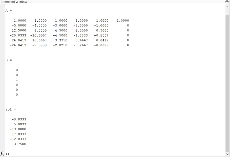
`[[1,1,1,1,1,1],[-5,-4,-3,-2,-1,0],[25/2,16/2,9/2,4/2,1/2,0],[-125/6,-64/6,-27/6,-8/6,-1/6,0],[625/24,256/24,81/24,16/24,1/24,0],[-3125/120,-1024/120,-243/120,-32/120,-1/120,0]]*[[a],[b],[c],[d],[e],[g]]=[[0],[0],[1],[0],[0],[0]`

Solving the above matrices using MATLAB to find the values of the coefficient

A=[1,1,1,1,1,1;-5,-4,-3,-2,-1,0;25/2,16/2,9/2,4/2,1/2,0;-125/6,-64/6,-27/6,-8/6,-1/6,0;625/24,256/24,81/24,16/24,1/24,0;-3125/120,-1024/120,-243/120,-32/120,-1/120,0]

B=[0;0;1;0;0;0]

sol=inv(A)*B

Matlab Coding

clear all
close all
clc
% f(x)=exp(x).cos(x)
%By using taylor table method finding the second order derivative for fourth order approximation
% Function, f(x) = exp(x).cos(x)
x = pi/3;
dx = linspace(pi/4000,pi/40,100);
% second order analytical derivative of the function
analytical_derivative = -2*exp(x)*sin(x);

% Central Differencing
a_central_differencing = [1 1 1 1 1;-2 -1 0 1 2;4/2 1/2 0 1/2 4/2;-8/6 -1/6 0 1/6 8/6;16/24 1/24 0 1/24 16/24];

b_central_differencing = [0;0;1;0;0];

c_central_differencing = inv(a_central_differencing) * b_central_differencing;

% Calculating second order numerical derivative using Central differencing
central_differencing = (c_central_differencing(1)*(exp(x-dx*2).*sin(x-dx*2)) + c_central_differencing(2)*(exp(x-dx).*sin(x-dx)) + c_central_differencing(3)*(exp(x).*sin(x)) + c_central_differencing(4).*(exp(x+dx).*sin(x+dx)) + c_central_differencing(5).*(exp(x+dx*2).*sin(x+dx*2)))./(dx.^2);

% Absolute error between second order derivative of analytical and central differencing scheme
central_error = abs(central_differencing - analytical_derivative);

%Right Sided Skewed
a_right_skewed = [1 1 1 1 1 1;0 1 2 3 4 5;0 1/2 4/2 9/2 16/2 25/2;0 1/6 8/6 27/6 64/6 125/6;0 1/24 16/24 81/24 256/24 625/24;0 1/120 32/120 243/120 1024/120 3125/120];

b_right_skewed = [0;0;1;0;0;0];

c_right_skewed = inv(a_right_skewed) * b_right_skewed;

% Calculating second order numerical derivative using Central differencing
right_skewed = (c_right_skewed(1).*(exp(x)*sin(x)) + c_right_skewed(2).*(exp(x+dx).*sin(x+dx)) + c_right_skewed(3).*(exp(x+2*dx).*sin(x+2*dx)) + c_right_skewed(4).*(exp(x+3*dx).*sin(x+3*dx)) + c_right_skewed(5).*(exp(x+4*dx).*sin(x+4*dx)) + c_right_skewed(6).*(exp(x+5*dx).*sin(x+5*dx)))./(dx.^2);

% Absolute error between second order derivative of analytical and skewed right-sided scheme
right_skewed_error = abs(right_skewed - analytical_derivative);

% Left Sided Skewed
a_left_skewed = [1 1 1 1 1 1;-5 -4 -3 -2 -1 0;25/2 16/2 9/2 4/2 1/2 0;-125/6 -64/6 -27/6 -8/6 -1/6 0;625/24 256/24 81/24 16/24 1/24 0;-3125/120 -1024/120 -243/120 -32/120 -1/120 0];

b_left_skewed = [0;0;1;0;0;0];

c_left_skewed = inv(a_left_skewed) * b_left_skewed;

% Calculating second order numerical derivative using Central differencing
left_skewed = (c_left_skewed(1).*(exp(x-5*dx).*sin(x-5*dx)) + c_left_skewed(2).*(exp(x-4*dx).*sin(x-4*dx)) + c_left_skewed(3).*(exp(x-3*dx).*sin(x-3*dx)) + c_left_skewed(4).*(exp(x-2*dx).*sin(x-2*dx)) + c_left_skewed(5).*(exp(x-dx).*sin(x-dx)) + c_left_skewed(6).*(exp(x)*sin(x)))./(dx.^2);

% Absolute error between second order derivative of analytical and skewed left-sided scheme
left_skewed_error = abs(left_skewed - analytical_derivative);

% Plotting the results
loglog(central_error,'b','linewidth',2);
grid on
hold on
loglog(right_skewed_error,'r','linewidth',2);
grid on
hold on
loglog(left_skewed_error,'c','linewidth',2);
grid on
hold off
xlabel('log dx')
ylabel('log Errors')
title('Error Evaluation')
legend('Central Differencing','Right-Sided Skewed','Left-Sided Skewed')

Grapg

Result

The central differencing scheme is morw accurate when compared to right & left skewed differencing.

Q) Why a skewed scheme is useful? What can a skewed scheme do that a CD scheme cannot?

ans) A skewed scheme is usful in initial and ending points like some cases 'Boundary conditions,Heat transfer impatc of stress at edges', where as centeral difference scheme will use both sides problems