Week 9 - FVM Literature Review

AIM :

• Define is Finite Volume Method (FVM).
• Write down the major difference between FDM & FVM
• Describe the need for interpolation schemes and flux limiters in FVM, with 1D linear heat conduction equation as an example.

Finite Volume Method :

• The Finite Volume method (FVM) is a discretization method for the approximation of a single or a system of partial differential equationsexpressing the conservation, or balance, of one or more quantities.

• These partial differential equations (PDEs) are often called conservation laws. They describe the relationship between partial derivatives of unknown fields such as temperature, concentration, pressure, molar fraction, density of electrons or probability density function, with respect to variables within the domain (space, time) under consideration.

• Therefore, the finite volume method is used by various numerical techniques in which the solution domain is descretised into a number of control volumes over which integrals of conservation laws are directly discretised.

Difference between FDM & FVM

• Finite difference method(FDM):

The grid is linear and aligned so that all grid points lie in a straight line . Main thing is that the properties are considered to concentrated at a

single point.

• Finite volume method(FVM):

The method is applied over a volume such that the governing equation is valid over the entire volume , aslo the properties are assumed to be

concentrated at the geometric centre of the volume concerned.

Need for Interpolation schemes :

Interpolation schemes is to find the value of properties at the boundaries of the control volumes.

To find out the value of thermal conductivity at a boundary of a control volume and if it a function of temperature we will have to interpolate

the values of the temperature from the neighbouring nodes to find the temperature at the boundary and that only we will be able to find the

value of thermal conductivity at that boundary.

Need for Flux Limiter:

While calculating the interpolations there might be sudden jump in the values of fluxes due to shocks in the system this can create errors

and may even blow up our solutions so to lime the values of fluxes we need to provide flux limiters.

Now let us take an example of 1D heat conduction equation to understand the FVM more clearly

We willbe considering a problem of a source free heat conduction in an insulated rod whose end are maintained at constant temperature 100 and 500 as shown in the figure.

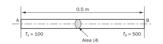
the governing equation for this 1D problem will be

`d/dx(kdt/dx) = 0`

Now we have to calculate the steady state temperature distribution in the rod.

considering the thermal consuctivity (k = 1000W/mK) and the cross sectional area (A = 10^-2 sq m).

after dividing the rod into 5 equal control volumes `delx=0.1`we will be discretising the equation.

considering nodal point 2 as our present node for the control volume be identifeid as P the point to its west can be identified as W and

similarly point east as E now the corresponding boundaries can be identified as 'w' and 'e' for west and east boundary.

applying integration on our governing equation over the control volume

`int_(DeltaV)d/dxk((dT)/(dx)) = kA((dT)/(dx))_e -kA((dT)/(dx))_w=0`