Week 5.1 - Mid term project - Solving the steady and unsteady 2D heat conduction problem
Aim:
Aim solve the 2D heat conduction equation by using the point iterative techniques that were taught in the class. The Boundary conditions for the problem are as follows;
Top Boundary = 600 K
Bottom Boundary = 900 K
Left Boundary = 400 K
Right Boundary = 800 K
You will implement the following methods for solving implicit equations.
1. Jacobi
2. Gauss-seidel
3. Successive over-relaxation
Your absolute error criteria are 1e-4.
Solution:
Here we are going to understand the concept of the 2d heat conduction equation of both stead and transient state of flow. We need to understand the derivation part where the terms are being discretized sequentially and then we move on to the coding part. There are few things that need to be considered before going over it is that for steady-state we need to apply iterative solvers and for transient, we have to solve both the schemes we seen in the previous section as IMPLICIT and EXPLICIT.
Now we are going to understand the derivation part of the steady-state condition.
Solving this by
1. Jacobi
2. Gauss-seidel
3. Successive Over Relaxation SOR
since d2t/dx2 + d2T/dy2 = 0, its has elliptic nature properties which we an discretize them using central differencing scheme
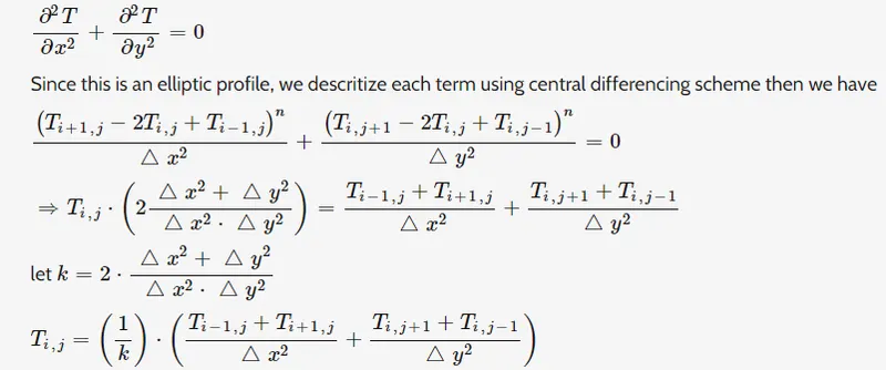
now what happens when represent them as jacobi

for Gauss seidel

and SOR is enhanced gauss-seidel method where nth time step and n+1 time step is all same.

where omega is the relaxation factor as 1.4.
now here we begin the coding part which is done in MATLAB where these all terms are considered by applying for loop and while loop.
Program of steady state 2D heat conduction equation.
1.1-Solving thru Jacobi, Gauss-Seidel (GS) & Successive Over Relaxation (SOR) Iteration method:
%% Script for solving 2d Steady state heat conduction eqn
close all
clear all
clc

%% Inputs
L=1; %length of domain is a unit square
%no of grid points along X & Y
nx=30;
ny=nx;
x=linspace(0,L,nx);
y=linspace(0,L,ny);
dx=x(2)-x(1);
dy= y(2)-y(1);
error = 9e9;
tol = 1e-4;
alpha=1.8;%For SOR
%% Defining boundary conditions
T_L = 400;
T_T = 600;
T_R = 800;
T_B = 900;
T = ones(nx,ny);
T(2:ny-1,1) = T_L;
T(2:ny-1,nx) = T_R;
T(1,2:nx-1) = T_T;
T(nx,2:ny-1) = T_B;

%% calculating average temperature at the matrix corners
T(1,1) = (T_T + T_L)/2;
T(nx,ny) = (T_R + T_B)/2;
T(1,ny) = (T_T + T_R)/2;
T(nx,1) = (T_L + T_B)/2;

%% other factors to be considered
[X,Y] = meshgrid(x,y);
Told = T;

%% Calculation of 2d Steady state heat conduction eqn
iterative_solver=1:3;
%% Jacobi Iteration
for iterative_solver=1
tic;
if iterative_solver==1
    jacobi_iter=1;
    while(error > tol)
        for i=2:nx-1
            for j=2:ny-1
                T(i,j) = 0.25*((Told(i-1,j)+Told(i+1,j)+Told(i,j-1)+Told(i,j+1)));
            end
        end
        error = max(max(abs(Told-T)));
        Told = T;
        jacobi_iter=jacobi_iter+1;
    end
end
F=toc;

%plot
figure(1)
[M,N]=contourf(X,Y,T);
clabel(M,N)
colormap(jet)
colorbar
title_text=sprintf(\'Jacobi Steady iteration number =%d ,Total Time F=%fs\',jacobi_iter,F);
title(title_text)
xlabel(\'X-axis\')
ylabel(\'Y-axis\')
fprintf(\'No of Iteration in jacobi=%d\\n\',jacobi_iter);
end

%% GS Iter
for iterative_solver=2
%update values
L=1;
nx=30;
ny=nx;
x=linspace(0,L,nx);
y=linspace(0,L,ny);
dx=x(2)-x(1);
dy= y(2)-y(1);
error = 9e9;
tol = 1e-4;
T_L = 400;
T_T = 600;
T_R = 800;
T_B = 900;
T = ones(nx,ny);
T(2:ny-1,1) = T_L;
T(2:ny-1,nx) = T_R;
T(1,2:nx-1) = T_T;
T(nx,2:ny-1) = T_B;
T(1,1) = (T_T + T_L)/2;
T(nx,ny) = (T_R + T_B)/2;
T(1,ny) = (T_T + T_R)/2;
T(nx,1) = (T_L + T_B)/2;
[X,Y] = meshgrid(x,y);
Told = T;

tic;
if iterative_solver==2
    GS_iter=1;
    while(error > tol)
        for i=2:nx-1
            for j=2:ny-1
                T(i,j) = 0.25*(T(i-1,j)+Told(i+1,j)+T(i,j-1)+Told(i,j+1));
            end
        end
        error = max(max(abs(Told-T)));
        Told = T;
        GS_iter=GS_iter+1;
    end
end
F=toc;

% plot
figure(2)
[M,N]=contourf(X,Y,T);
clabel(M,N)
colormap(jet)
colorbar
title_text=sprintf(\'GS steady iteration number =%d ,Total Time F=%fs\',GS_iter,F);
title(title_text)
xlabel(\'X-axis\')
ylabel(\'Y-axis\')
fprintf(\'No of Iteration in GS=%d\\n\',GS_iter);
end

%% SOR Iter
for iterative_solver=3
%update values
L=1;
nx=30;
ny=nx;
x=linspace(0,L,nx);
y=linspace(0,L,ny);
dx=x(2)-x(1);
dy= y(2)-y(1);
error = 9e9;
tol = 1e-4;
T_L = 400;
T_T = 600;
T_R = 800;
T_B = 900;
T = ones(nx,ny);
T(2:ny-1,1) = T_L;
T(2:ny-1,nx) = T_R;
T(1,2:nx-1) = T_T;
T(nx,2:ny-1) = T_B;
T(1,1) = (T_T + T_L)/2;
T(nx,ny) = (T_R + T_B)/2;
T(1,ny) = (T_T + T_R)/2;
T(nx,1) = (T_L + T_B)/2;
[X,Y] = meshgrid(x,y);
Told = T;

tic;
if iterative_solver==3
    SOR_iter=1;
    while(error > tol)
        for i=2:nx-1
            for j=2:ny-1
                T(i,j) = ((1-alpha)*Told(i,j)+(alpha*0.25*(T(i,j-1)+Told(i,j+1)+T(i-1,j)+Told(i+1,j))));
            end
        end
        error = max(max(abs(Told-T)));
        Told = T;
        SOR_iter=SOR_iter+1;
    end
end
F=toc;

% plot
figure(3)
[M,N]=contourf(X,Y,T);
clabel(M,N)
colormap(jet)
colorbar
title_text=sprintf(\'SOR steady iteration number =%d ,Total Time F=%fs\',SOR_iter,F);
title(title_text)
xlabel(\'X-axis\')
ylabel(\'Y-axis\')
fprintf(\'No of Iteration in SOR=%d\\n\',SOR_iter);
end
%% END
1.2-Steady State Program Output:
2-For Unsteady State Flow:
The generalised 2D temperature Equation is,
α(∂2T∂x2+α∂2T∂y2)=∂T∂tα(∂2T∂x2+α∂2T∂y2)=∂T∂t
We discretize the eqn by Central Differencing & time gradient Eqn with Forward Differencing Method
- The Eqn with respect to X becomes,
∂2T∂x2=T(i−1,j)−2T(i,j)+T(i+1,j)Δx2∂2T∂x2=T(i−1,j)−2T(i,j)+T(i+1,j)Δx2
- The Eqn with respect to Y becomes,
∂2T∂y2=T(i,j−1)−2T(i,j)+T(i,j+1)Δy2∂2T∂y2=T(i,j-1)−2T(i,j)+T(i,j+1)Δy2
- The Eqn with respect to time gradient becomes
∂T∂t=Tn+1(i,j)−Tn(i,j)Δt∂T∂t=Tn+1(i,j)−Tn(i,j)Δt
We can define 2 constants namely k1 and k2
k1=αΔtΔx2k1=αΔtΔx2
k2=αΔtΔy2k2=αΔtΔy2
Since we assumed nx=ny then we can take Δx2=Δy2Δx2=Δy2
then the Eqn becomes as
Tn+1(i,j)=Tn(i,j)+k1(T(i−1,j)+T(i+1,j))n+1+k2(T(i,j−1)+T(i,j+1))n+11+2K4+2K5Tn+1(i,j)=Tn(i,j)+k1(T(i−1,j)+T(i+1,j))n+1+k2(T(i,j−1)+T(i,j+1))n+11+2K4+2K5
2.1.1-Solving Transient Flow(Explicit):
%% Script for solving 2d Transient state heat conduction eqn(Explicit)
close all
clear all
clc

%% Inputs
L=1; %length of domain is a unit square
%no of grid points along X & Y
nx=30;
ny=nx;
x=linspace(0,L,nx);
y=linspace(0,L,ny);
dx=x(2)-x(1);
dy= y(2)-y(1);
error = 9e9;
tol = 1e-4;
dt = 0.01;
alpha=1.88e-5;%thermal diffusivity for steel
%% Defining boundary conditions
T_L = 400;
T_T = 600;
T_R = 800;
T_B = 900;
T = ones(nx,ny);
T(2:ny-1,1) = T_L;
T(2:ny-1,nx) = T_R;
T(1,2:nx-1) = T_T;
T(nx,2:ny-1) = T_B;

%% calculating average temperature at the matrix corners
T(1,1) = (T_T + T_L)/2;
T(nx,ny) = (T_R + T_B)/2;
T(1,ny) = (T_T + T_R)/2;
T(nx,1) = (T_L + T_B)/2;

%% other factors to be considered
%we know the values for constants k
k1 = (alpha*dt)/(dx^2);
k2 = (alpha*dt)/(dy^2);
[X,Y] = meshgrid(x,y);
Told = T;

%% Calculation of 2d Transient state heat conduction eqn in Explicit
iterative_solver=1;
tic;
if iterative_solver==1
    solver_counter=1;
    while(error > tol)
        for i=2:nx-1
            for j=2:ny-1
                term1 = Told(i,j);
                term2 = k1*(Told(i+1,j)-2*Told(i,j)+Told(i-1,j));
                term3 = k2*(Told(i,j+1)-2*Told(i,j)+Told(i,j-1));
                T(i,j)= term1+term2+term3 ;
            end
        end
        error = max(max(abs(Told-T)));
        Told = T;
        solver_counter=solver_counter+1;
    end
end
F=toc;

%% plot
figure(1)
[M,N]=contourf(X,Y,T);
clabel(M,N)
colormap(jet)
colorbar
title_text=sprintf(\'Transient iteration number thru explicit=%d ,Total Time F=%fs\',solver_counter,F);
title(title_text)
xlabel(\'X-axis\')
ylabel(\'Y-axis\')
fprintf(\'No of Iteration in Transient(explicit)=%d\\n\',solver_counter);
%% END
2.1.2-Transient Flow(Explicit) Output:
2.2.1-Solving Transient Flow(Implicit-Jacobi, GS & SOR):
%% Script for solving 2d Transient state heat conduction eqn(Implicit)
close all
clear all
clc

%% Inputs
L=1; %length of domain is a unit square
%no of grid points along X & Y
nx=30;
ny=nx;
x=linspace(0,L,nx);
y=linspace(0,L,ny);
dx=x(2)-x(1);
dy= y(2)-y(1);
error = 9e9;
tol = 1e-4;
dt = 2000;
alpha=1.88e-5;%thermal diffusivity for steel
alpha1=1.8;%For SOR
%% Defining boundary conditions
T_L = 400;
T_T = 600;
T_R = 800;
T_B = 900;
T = ones(nx,ny);
T(2:ny-1,1) = T_L;
T(2:ny-1,nx) = T_R;
T(1,2:nx-1) = T_T;
T(nx,2:ny-1) = T_B;

%% calculating average temperature at the matrix corners
T(1,1) = (T_T + T_L)/2;
T(nx,ny) = (T_R + T_B)/2;
T(1,ny) = (T_T + T_R)/2;
T(nx,1) = (T_L + T_B)/2;

%% other factors to be considered
%we know the values for constants k
k1 = (alpha*dt)/(dx^2);
k2 = (alpha*dt)/(dy^2);
[X,Y] = meshgrid(x,y);
Told = T;
T_Prev_dt = Told;

%% Calculation of 2d Transient state heat conduction eqn(Implicit)
iterative_solver=1:3;
%% Jacobi Iteration
term1=(1+2*k1+2*k2)^(-1);
term2=k1*term1;
term3=k2*term1;
for iterative_solver=1
tic;
if iterative_solver==1
    jacobi_iter=1;
    while(error > tol)
        for i=2:nx-1
            for j=2:ny-1
                H = (Told(i-1,j)+Told(i+1,j));
                V = (Told(i,j-1)+Told(i,j+1));
                T(i,j) = term1*T_Prev_dt(i,j)+term2*H+term3*V;
            end
        end
        error = max(max(abs(Told-T)));
        Told = T;
        jacobi_iter=jacobi_iter+1;
    end
end
F=toc;

%plot
figure(1)
[M,N]=contourf(X,Y,T);
clabel(M,N)
colormap(jet)
colorbar
title_text=sprintf(\'Jacobi UnSteady(Implicit) iteration number =%d ,Total Time F=%fs\',jacobi_iter,F);
title(title_text)
xlabel(\'X-axis\')
ylabel(\'Y-axis\')
fprintf(\'No of Iteration in jacobi=%d\\n\',jacobi_iter);
end

%% GS Iter
%update values
L=1;
nx=30;
ny=nx;
x=linspace(0,L,nx);
y=linspace(0,L,ny);
dx=x(2)-x(1);
dy= y(2)-y(1);
error = 9e9;
tol = 1e-4;
dt = 2000;
alpha=1.88e-5;%thermal diffusivity for steel
T_L = 400;
T_T = 600;
T_R = 800;
T_B = 900;
T = ones(nx,ny);
T(2:ny-1,1) = T_L;
T(2:ny-1,nx) = T_R;
T(1,2:nx-1) = T_T;
T(nx,2:ny-1) = T_B;
T(1,1) = (T_T + T_L)/2;
T(nx,ny) = (T_R + T_B)/2;
T(1,ny) = (T_T + T_R)/2;
T(nx,1) = (T_L + T_B)/2;
k1 = (alpha*dt)/(dx^2);
k2 = (alpha*dt)/(dy^2);
[X,Y] = meshgrid(x,y);
Told = T;
T_Prev_dt = Told;

term1 = (1+2*k1+2*k2)^(-1);
term2 = k1*term1;
term3 = k2*term1;
for iterative_solver=2
tic;
if iterative_solver==2
    GS_iter=1;
    while(error > tol)
        for i=2:nx-1
            for j=2:ny-1
                H = (T(i-1,j)+Told(i+1,j));
                V = (T(i,j-1)+Told(i,j+1));
                T(i,j) = term1*T_Prev_dt(i,j)+term2*H+term3*V;
            end
        end
        error = max(max(abs(Told-T)));
        Told = T;
        GS_iter=GS_iter+1;
    end
end
F=toc;

% plot
figure(2)
[M,N]=contourf(X,Y,T);
clabel(M,N)
colormap(jet)
colorbar
title_text=sprintf(\'GS Transient(Implicit) iteration number =%d ,Total Time F=%fs\',GS_iter,F);
title(title_text)
xlabel(\'X-axis\')
ylabel(\'Y-axis\')
fprintf(\'No of Iteration in GS=%d\\n\',GS_iter);
end

%% SOR Iter
%update values
L=1;
nx=30;
ny=nx;
x=linspace(0,L,nx);
y=linspace(0,L,ny);
dx=x(2)-x(1);
dy= y(2)-y(1);
error = 9e9;
tol = 1e-4;
dt = 2000;
alpha=1.88e-5;%thermal diffusivity for steel
T_L = 400;
T_T = 600;
T_R = 800;
T_B = 900;
T = ones(nx,ny);
T(2:ny-1,1) = T_L;
T(2:ny-1,nx) = T_R;
T(1,2:nx-1) = T_T;
T(nx,2:ny-1) = T_B;
T(1,1) = (T_T + T_L)/2;
T(nx,ny) = (T_R + T_B)/2;
T(1,ny) = (T_T + T_R)/2;
T(nx,1) = (T_L + T_B)/2;
k1 = (alpha*dt)/(dx^2);
k2 = (alpha*dt)/(dy^2);
[X,Y] = meshgrid(x,y);
Told = T;
T_Prev_dt = Told;

term1 = (1+2*k1+2*k2)^(-1);
term2 = k1*term1;
term3 = k2*term1;
for iterative_solver=3
tic;
if iterative_solver==3
    SOR_iter=1;
    while(error > tol)
        for i=2:nx-1
            for j=2:ny-1
                H=(alpha1*T(i-1,j)+(1-alpha1)*Told(i-1,j)+Told(i+1,j));
                V=(alpha1*T(i,j-1)+(1-alpha1)*Told(i,j-1)+Told(i,j+1));
                T(i,j)=T_Prev_dt(i,j)*term1+(term2*H+term3*V);
            end
        end
        error = max(max(abs(Told-T)));
        Told = T;
        SOR_iter=SOR_iter+1;
    end
end
F=toc;

% plot
figure(3)
[M,N]=contourf(X,Y,T);
clabel(M,N)
colormap(jet)
colorbar
title_text=sprintf(\'SOR Transient(Implicit) iteration number =%d ,Total Time F=%fs\',SOR_iter,F);
title(title_text)
xlabel(\'X-axis\')
ylabel(\'Y-axis\')
fprintf(\'No of Iteration in SOR=%d\\n\',SOR_iter);
end
%% END