Week 5.1 - Mid term project - Solving the steady and unsteady 2D heat conduction problem
OBJECTIVE:
To solve Steady and Unsteady state 2D Heat Conduction Equation by using the point iterative techniques such as Jacobi, Gauss Seidel & Successive over-relaxation for both implicit and explicit schemes using MATLAB.
Assumptions:-
- Area to be computed is square with unit Length.
- Assume nx = ny=10,i.e No. of points on x-direction is equal to no. of points in y-direction]
- Boundary Conditions are
Temperature at Left Boundry = 400K
Temperature at Right Boundry = 800K
Temperature at Top Boundry = 600K
Temperature at Bottom Boundry = 900K
and all other nodes are assumed having initial temperature of 300K.
Various methods to be employed in solving the steady state,unsteady/ Transient states are:-
Jacobi, Gauss Scidel, successive Over Relaxation (S.O.R).
Introduction
The 2-D heat conduction equation is a partial differential equation which governs the heat transfer through a medium by thermal conduction. The equation is defined as:
`(∂T)/(∂t)=α[(∂^2T)/(∂x^2)+(∂^2T)/(∂y^2)]`
For the steady state, the temperature does not vary with time, hence the time differential is equal to 0. The equation then gets modified to:
`[(∂^2T)/(∂x^2)+(∂^2T)/(∂y^2)]=0`
Here, α is the thermal diffusivity which is characteristic for a medium.
The domain over which the above equation is solved is a square domain with unit length. It is divided into small elements to implement the discretized schemes. so, it is divided into an equal number of elements in the x and y directions (nx=ny). The domain also has specified boundary conditions in order to obtain a solution to the heat conduction equation.
Boundary Conditions are:-
Temperature at Left Boundry = 400K
Temperature at Right Boundry = 800K
Temperature at Top Boundry = 600K
Temperature at Bottom Boundry = 900K
The values at the corner nodes are taken as the average of the values from the surrounding edges. The equation is solved for steady and unsteady/transient state separately. Each point which is being solved takes information from its surrounding nodes.
Working of program loops:-
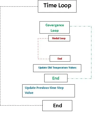
STEADY STATE:
The steady state equation is discretized using the central difference scheme in both x
and y directions. Suppose i and j are the node numbers in the x and y
directions respectively, then
`[(∂^2T)/(∂x^2)+(∂^2T)/(∂y^2)]=0`
`(T_(i−1,j)-2*T_(i,j)+T_(i+1,j))/(dx)^2+(T_(i,j-1)-2*T_(i,j)+T_(i,j+1))/(dy)^2=0`
Hence this Equation will be used to get solution for a steady state
`T_p=T_(i,j)=(1/k)*((T_(i−1,j)+T_(i+1,j))/(dx)^2+(T_(i,j-1)+T_(i,j+1))/(dy)^2)`
Where `k= 2*((delx^2+ dely^2)/(delx^2* dely^2))`
This is the final equation that needs to be solved. We use three iterative solvers for the above equation, namely - Jacobi, Gauss-Seidel and Successive Over-Relaxation (SOR). Each of the solvers solves the equation iteratively until the iterative error falls below the specified tolerance value, which is 1e-4 (`10^-4`)
In this case. The difference between the methods is the manner in which the values for the successive iterations are updated through the values from the previous iterations.
For the Jacobi solver, all the values in the RHS are taken from the previous iteration (previous Temp. values).
the following equation denotes the iteration number.
`T(i,j)^(n+1)=(1/k)*((Told_(i-1,j)+Told_(i+1,j))/(dx^2)+(Told_(i,j-1)+Told_(i,j+1))/(dy^2))^n`
Where, `k= 2*((delx^2+ dely^2)/(delx^2* dely^2))`
For the Gauss-Seidel solver, the values that have already been updated in the current iteration are used and the rest of the values are taken from the previous iteration.
`T(i,j)^(n+1)=(1/k)*((T_(i-1,j)+T_(i+1,j))/(dx^2)+(T_(i,j-1)+T_(i,j+1))/(dy^2))^(n+1)`
Where, `k= 2*((delx^2+ dely^2)/(delx^2* dely^2))`
The SOR solver is a modification of the Gauss-Seidel solver in which the values are updated according to the relaxation paramater. The relaxation parameter can take a range of values 0<ω<2
which determine whether the solver is over-relaxed or under-relaxed.
If ω<1, called as under relaxed
ω >1, called as over relaxed
`T_(i,j)^(n+1)=(1-omega)*Told_(i,j)+omega*T_(i,j)`
`T(i,j)^(n+1)=(1/k)*((T_(i-1,j)+T_(i+1,j))/(dx^2)+(T_(i,j-1)+T_(i,j+1))/(dy^2))^(n+1)`
Where, `k= 2*((delx^2+ dely^2)/(delx^2* dely^2))`The above solvers are implemented in MATLAB for the defined domain, and the steady state results are compared.
STEADY STATE MATLAB CODE AND RESULTS:
The code asks for the selection of the iterative solver in command window. Once selected, the code runs that solver and outputs the result. If no selection is made, the program exits by itself. The code also calculates and record the error during each iteration, which is defined as the maximum absolute difference in the temperature in this iteration and the temperature from the previous iteration (change in temperature within iterations). The number of iterations taken by each solver to converge is also recorded .
clear all
close all
clc
%% inputs
TT=600;
TB= 900;
TL= 400;
TR= 800;
%tol is the point at which our solution assumed to be converged.
tol =1e-4;
error=9e9;
% no. of Rows is nx for Temperature Array
nx=10;
% no. of Columns is ny for Temperature Array
ny=nx;
x=linspace(0,1,nx);
y=linspace(0,1,ny);
% Grid step size dx & dy
dx=x(2)-x(1);
dy=y(2)-y(1);
% assuming Initial Temperature is 300K
T=300*ones(nx,ny);

%assigning B.C
T(2:nx-1,1)=TL;
T(2:nx-1,ny)=TR;
T(1,2:ny-1)=TT;
T(ny,2:ny-1)=TB;
% avg. Temperature at Corners
T(1,1)=(TL+TT)*0.5;
T(nx,1)=(TL+TB)*0.5;
T(1,ny)=(TR+TT)*0.5;
T(nx,ny)=(TR+TB)*0.5;
% creating  copies of T Temperature
Told=T;
Tinit=T;
omega=1.2;
iterative_solver=input('Enter 1 for Jacobi, 2 for Gauss scidel, 3 for S.O.R iterative Method:- ');
K=2*((dx^2)+(dy^2))/((dx^2)*(dy^2));
%% Steady State Heat Conduction Equation using Jacobi Iteration
if iterative_solver==1
    jacobi_iter=1;
    while(error>tol)
        for i=2:nx-1
            for j=2:ny-1
                T(i,j)=(1/K)*((Told(i-1,j)+Told(i+1,j))/(dx^2)+(Told(i,j-1)+Told(i,j+1))/(dy^2));
            end
        end
        error=max(max(abs(Told-T)));
        Told=T;
        jacobi_iter=jacobi_iter+1;
    end
    %Plotting
    figure(1)
    contourf(x,y,T)
    clabel(contourf(x,y,T))
    colorbar
    colormap(jet)
    set(gca,'ydir','reverse')
    title(sprintf('No. of Jacobi iterations in steady state '),jacobi_iter)
    xlabel('X Axis')
    ylabel('Y Axis')
end
%% Steady State Heat Conduction Equation using Gauss scidel_iteration
if iterative_solver==2
    Gauss_iter=1;
    while(error>tol)
        for i=2:nx-1
            for j=2:ny-1
                T(i,j)=(1/K)*((T(i-1,j)+T(i+1,j))/(dx^2)+(T(i,j-1)+T(i,j+1))/(dy^2));
            end
        end
        error=max(max(abs(Told-T)));
        Told=T;
        Gauss_iter=Gauss_iter+1;
    end
    %Plotting
    figure(2)
    contourf(x,y,T)
    clabel(contourf(x,y,T))
    colorbar
    colormap(jet)
    set(gca,'ydir','reverse')
    title_text='No. of Gauss iterations in steady state ';
    title(title_text,Gauss_iter);
    xlabel('X Axis')
    ylabel('Y Axis')
end
%% Steady State Heat Conduction Equation using Successive Over relaxation (S.O.R) Iteration
if iterative_solver==3
  SOR_iter=1;
    while(error>tol)
        for i=2:nx-1
            for j=2:ny-1
                T(i,j)=(1/K)*((T(i-1,j)+T(i+1,j))/(dx^2)+(T(i,j-1)+T(i,j+1))/(dy^2));
                T(i,j)=(1-omega)*Told(i,j)+omega*T(i,j);
            end
        end
        error=max(max(abs(Told-T)));
        Told=T;
        SOR_iter=SOR_iter+1;
    end
    %Plotting
    figure(3)
    contourf(x,y,T)
    clabel(contourf(x,y,T))
    colorbar
    colormap(jet)
    set(gca,'ydir','reverse')
    title_text='No. of SOR iterations  in steady state ';
    title(title_text,SOR_iter);
    xlabel('X Axis')
    ylabel('Y Axis')
end

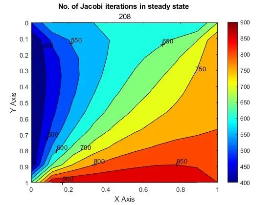
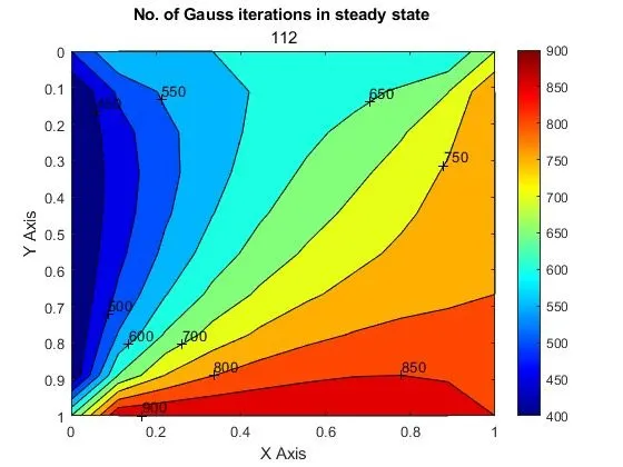
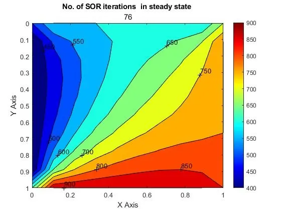
No. of jacobi iteration>No. of Gauss Scidel iteration>No. of S.O.R iteration
TRANSIENT STATE (EXPLICIT):-
In the transient equation, the time derivative does not disappear and we use the entire heat conduction equation. We discretize the time derivative using forward difference scheme. The transient scheme can be implicit or explicit depending on the time-step at which the spatial derivatives are chosen. First, we will focus on the explicit scheme where all the spatial derivatives are taken from the previous time step. The heat conduction equation, after discretization, modifies to:
`(T_(i,j)^(n+1)−T_(i,j)^n)/(Δt) = α[(T_(i−1,j)^n−2*T_(i,j)+T_(i+1,j)^n)/(Δx)^2+(T_(i,j-1)^n−2*T_(i,j)+T_(i,j+1)^n)/(Δy)^2]`
`T_(i,j)^(n+1)=(1/(1+2*k1+2*k2))*(Told_(i,j)+(k1*(Told_(i-1,j)+Told_(i+1,j)))+k2*(Told_(i,j-1)+Told_(i,j+1)))`
Here Told represents the previous time step temperature.
For the purpose of stability, the CFL no. >1 is chosen for the explicit solver.
TRANSIENT STATE (IMPLICIT):
For the implicit solver, the terms Ti,j
on the RHS are taken at the time-step n+1 as opposed to n
in the explicit solver. This changes the discretization of the transient equation to
`T_(i,j)^(n+1)=T_(i,j)^n+αΔt((T_(i−1,j)^(n+1)+T_(i+1,j)^(n+1)-2*T_(i,j)^(n+1))/ (Δx^2))+((T_(i,j-1)^(n+1)+T_(i,j+1)^(n+1)-2*T_(i,j)^(n+1))/ (Δy^2))`
Substituting `k1=α(Δt)/ (Δx^2)`
`k2=α(Δt)/ (Δy^2)`
`T_(i,j)^(n+1)=T_(i,j)^n+k1*(T_(i−1,j)^(n+1)+T_(i+1,j)^(n+1)-2*T_(i,j)^(n+1))+k2*(T_(i,j-1)^(n+1)+T_(i,j+1)^(n+1)-2*T_(i,j)^(n+1))`
On solving
`T_(i,j)^(n+1)=(1/(1+2*k1+2*k2))*(T_(i,j)^n+k1*(T_(i−1,j)^(n+1)+T_(i+1,j)^(n+1))+k2*(T_(i,j-1)^(n+1)+T_(i,j+1)^(n+1)))`
on the RHS can never be negative. Hence, the implicit scheme is unconditionally stable for any value of k1 & k2
. Since the values on the RHS are also unknowns, we use iterative solvers to implicitly solve the heat conduction equation. The iterative solvers - Jacobi, Gauss-Seidel, and SOR, are used similarly as described in the steady-state section.
For Jacobi method,
`T_(i,j)^(n+1)=(1/(1+2*k1+2*k2))*(T_Init_(i,j)+(k1*(Told_(i-1,j)+Told_(i+1,j)))+k2*(Told_(i,j-1)+Told_(i,j+1)))`
Where Tinit (T(i,j)) and Told are previous time step temperatures for nth time step
For Gauss-Seidel method,
`T_(i,j)^(n+1)=(1/(1+2*k1+2*k2))*(T_Init_(i,j)+(k1*(T_(i-1,j)+T_(i+1,j)))+k2*(T_(i,j-1)+T_(i,j+1)))`
Where Tinit is n time step Temperature T(i,j) ,
T is the n+1 Time step temperature.
For SOR method,
T(i,j)=(1-omega)*Told(i,j)+omega*T(i,j);
Where, T(i,j)
`T_(i,j)^(n+1)=(1/(1+2*k1+2*k2))*(T_Init_(i,j)+(k1*(T_(i-1,j)+T_(i+1,j)))+k2*(T_(i,j-1)+T_(i,j+1)))`
Where Tinit is n time step temperature T(i,j) ,
T is the n+1 Time step temperature.
UNSTEADY TRANSIENT STATE MATLAB CODE AND RESULTS:
The code asks for the selection of the iterative solver in command window i.e Enter 1 for Jacobi, 2 for Gauss scidel, 3 for S.O.R iterative Method, 4 for Explicit Scheme. Once selected, the code runs that solver and outputs the result. If no selection is made, the program exits by itself. The code also calculates and record the error during each iteration, code will be in loop until error is less than tolerance value. The number of iterations taken by each solver to converge is also recorded .
%% Unsteady State Heat
clear all
close all
clc
%% inputs
TT=600;
TB= 900;
TL= 400;
TR= 800;
%tol is the point at which our solution assumed to be converged.
tol =1e-4;
error=9e9;
dT=1e-3;
% no. of Rows is nx for Temperature Array
nx=10;
% no. of Columns is ny for Temperature Array
ny=nx;
x=linspace(0,1,nx);
y=linspace(0,1,ny);
%[xx,yy]=meshgrid(x,y);
dx=x(2)-x(1);
dy=y(2)-y(1);
% assuming Initial Temperature is 300K
T=300*ones(nx,ny);
%assigning B.C
T(2:nx-1,1)=TL;
T(2:nx-1,ny)=TR;
T(1,2:ny-1)=TT;
T(ny,2:ny-1)=TB;
% avg. Temperature at Corners
T(1,1)=(TL+TT)*0.5;
T(nx,1)=(TL+TB)*0.5;
T(1,ny)=(TR+TT)*0.5;
T(nx,ny)=(TR+TB)*0.5;
% creating  copies of T Temperature
Told=T;
Tinit=T;
omega=1.1;
alpha=1.1;
nt=1400;
iterative_solver=input('Enter 1 for Jacobi, 2 for Gauss seidel, 3 for S.O.R iterative Method, 4 for Explicit Scheme :- ');
k1=alpha*(dT/dx^2);
k2=alpha*(dT/dy^2);
%% UnSteady State Heat Conduction Equation using Jacobi Iteration
if iterative_solver==1
    jacobi_iter=1;
    for l=1:nt
        error=9e9;
        while(error>tol)
            for i=2:nx-1
                for j=2:ny-1
                    T(i,j)=((1+2*k1+2*k2)^-1)*(Tinit(i,j)+(k1*(Told(i-1,j)+Told(i+1,j)))+k2*(Told(i,j-1)+Told(i,j+1)));
                end
            end
            error=max(max(abs(Told-T)));
            Told=T;
            jacobi_iter=jacobi_iter+1;
        end
        Tinit=T;
    end
    %Plotting
    figure(1)
    contourf(x,y,T)
    clabel(contourf(x,y,T))
    colorbar
    colormap(jet)
    set(gca,'ydir','reverse')
    title_text='No. of Jacobi iterations (Implicit) in unsteady state ';
    title(title_text,jacobi_iter)
    xlabel('X Axis')
    ylabel('Y Axis')
end


%% Steady State Heat Conduction Equation using Gauss seidel_iteration
if iterative_solver==2
    Gauss_iter=1;
    for l=1:nt
        error=9e9;
        while(error>tol)
            for i=2:nx-1
                for j=2:ny-1
                    T(i,j)=((1+2*k1+2*k2)^-1)*(Tinit(i,j)+(k1*(T(i-1,j)+T(i+1,j)))+k2*(T(i,j-1)+T(i,j+1)));
                end
            end
            error=max(max(abs(Told-T)));
            Told=T;
            Gauss_iter=Gauss_iter+1;
        end
        Tinit=T;
    end
    %Plotting
    figure(2)
    contourf(x,y,T)
    clabel(contourf(x,y,T))
    colorbar
    colormap(jet)
    set(gca,'ydir','reverse')
    title_text='No. of Gauss iterations (Implicit) in unsteady state ';
    title(title_text,Gauss_iter);
    xlabel('X Axis')
    ylabel('Y Axis')

end
%%Steady State Heat Conduction Equation using Successive Over relaxation (S.O.R) Iteration
if iterative_solver==3
    SOR_iter=1;
    for l=1:nt
        error=9e9;
        while(error>tol)
            for i=2:nx-1
                for j=2:ny-1
                    T(i,j)=((1+2*k1+2*k2)^-1)*(Tinit(i,j)+(k1*(T(i-1,j)+T(i+1,j)))+k2*(T(i,j-1)+T(i,j+1)));
                    T(i,j)=(1-omega)*Told(i,j)+omega*T(i,j);
                end
            end
            error=max(max(abs(Told-T)));
            Told=T;
            SOR_iter=SOR_iter+1;
        end
        Tinit=T;
    end
    %Plotting
    figure(3)
    contourf(x,y,T)
    clabel(contourf(x,y,T))
    colorbar
    colormap(jet)
    set(gca,'ydir','reverse')
    title_text='No. of SOR iterations (Implicit) in unsteady state ';
    title(title_text,SOR_iter);
    xlabel('X Axis')
    ylabel('Y Axis')
end
%% Steady State Heat Conduction Equation using Explicit Scheme
if iterative_solver==4
    iter=1;
    while(error>tol)
        for i=2:nx-1
            for j=2:ny-1
                T(i,j)=((1+2*k1+2*k2)^-1)*(Told(i,j)+(k1*(Told(i-1,j)+Told(i+1,j)))+k2*(Told(i,j-1)+Told(i,j+1)));
            end
        end
        error=max(max(abs(Told-T)));
        Told=T;
        iter=iter+1;
    end
    %Plotting
    figure(4)
    contourf(x,y,T)
    clabel(contourf(x,y,T))
    colorbar
    colormap(jet)
    set(gca,'ydir','reverse')
    title_text='No. of iteration in Explicit scheme in unsteady state ';
    title(title_text,iter);
    xlabel('X Axis')
    ylabel('Y Axis')
end

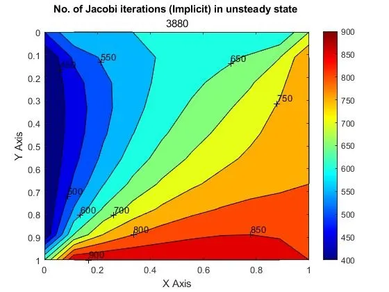

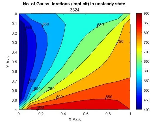

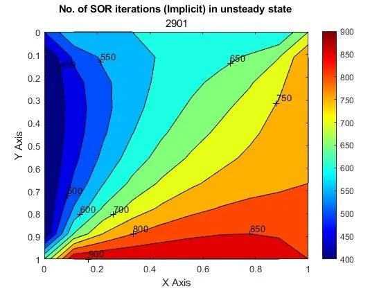

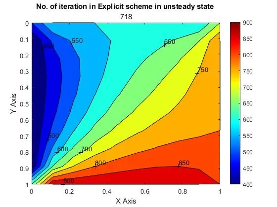
The explicit method is also fast in this case (718 iterations) since it is a 2-D equation on a simple domain, however for complex 3-D domains, it might be costlier than the implicit scheme. This is because of the restriction on the time-step for the explicit scheme.
CONCLUSION:-
| Type of scheme & analysis | Various Methods | No. of Iterations |
| steady State analysis |
Jacobi Gauss Seidel Successive Over Relaxation |
208 112 76 |
| Implicit Transient/unsteady State analysis |
Jacobi Gauss Seidel Successive Over Relaxation |
3380 3324 2901 |
| Explicit analysis | 718 |
From the finite difference formulations, it is evident that the Jacobi solver would be the slowest one as it updates the current iteration with all the values from the previous iteration, and Gauss-Seidel updates the current iteration with some values already calculated in the current iteration. The SOR method provides a greater edge over the Gauss-Seidel method as it determines how aggressively the current iteration gets updated from the values in the current iteration, which makes it much more faster than the normal Gauss-Seidel method.
1. Jacobi > Gauss-seidel > Successive over-relaxation according to the No. of iterations computed for all methods & Schemes.
2. When comparing Steady state and Unsteady state, it is proven that Steady state is the most successful one as it takes least number of iterations and least time to compute.
3. SOR iteration method is the most effective iteration method as it took least No. of iterations for coverging solutions in both the schemes (EXPLICIT & IMPLICIT) compared to Jacobi & Gauss-siedel.