Aim :
Steady state analysis & Transient State Analysis
Solve the 2D heat conduction equation by using the point iterative techniques that were taught in the class. The Boundary conditions for the problem are as follows;
Top Boundary = 600 K
Bottom Boundary = 900 K
Left Boundary = 400 K
Right Boundary = 800 K
You will implement the following methods for solving implicit equations.
1. Jacobi
2. Gauss-seidel
3. Successive over-relaxation
Your absolute error criteria is 1e-4
2. You will write code for both implicit and explicit schemes (This is for the Transient Analysis only)
3. Write a detailed explanation for your results, plots or codes without explanation will awarded zero marks.
Matlab code :
% Sloving the steady state analysis of 2D heat conduction equation
clear all
close all
clc
%Defining the inputs as given in the question
%length of domain
L=1;
nx = 10;
ny = 10;
x = linspace(0,1,nx);
y = linspace(0,1,ny);
%defining the distance between the nodes
dx = x(2)-x(1);
dy = y(2)-y(1);
%defining the boundary conditions
t = 300*ones(nx,ny);
t(1,:) = 600;
t(nx,:) = 900;
t(:,ny) = 800;
t(:,1) = 400;
% defining the corners points of the temperature
t(1,1) = 500;
t(1,ny) = 700;
t(nx,1) = 650;
t(nx, ny) = 850;
%defining the old value
t_old = t;
%t_prev = t;
%defining the error
error = 100;
%defining the tolerance as given in the question
tol = 1e-4;
%defining the constant value which we get in the wquation
k = 2*(dx^2+dy^2)/(dx^2*dy^2);
%defining the iterative value
method = input('iterative_method = ');
%jocobiean method of solving the equation
if(method == 1)
tic;
jocobi = 1;
while(error>tol)
for i = 2:nx-1
for j = 2:ny-1
t(i,j) = (((t_old(i-1,j)+t_old(i+1,j))/(dx^2))+((t_old(i,j-1)+t_old(i,j+1))/(dy^2)))/k;
end
end
error = max(max(abs(t-t_old)));
t_old=t;
jocobi = jocobi+1;
time_step = toc;
end
%plotting the figure
figure(1)
contourf(x,y,t, 'ShowText','on')
colormap("jet")
colorbar
xlabel('x')
ylabel('y')
text_1 = sprintf('number of iterstive = %d',jocobi);
text_2 = sprintf('stimulation of time = %f',time_step);
title({'steady state analysis jocobi';text_1;text_2});
end
% solving isung guass side1 method
if (method == 2)
tic;
guass=1;
while(error>tol)
for i = 2:nx-1
for j = 2:ny-1
t(i,j) = (((t(i-1,j)+t_old(i+1,j))/(dx^2))+((t(i,j-1)+t_old(i,j+1))/(dy^2)))/k;
end
end
error=max(max(abs(t-t_old)));
t_old=t;
guass=guass+1;
time_step = toc;
end
% plotting the figure
figure(2)
contourf(x,y,t,'ShowText','on')
colormap("jet")
colorbar
xlabel('x')
ylabel('y')
text_1 = sprintf('number of iteretive = %d',guass);
text_2 = sprintf('stimulation of time = %f',time_step);
title({'steady state analysis guass';text_1;text_2});
end
%solving using the succesive over relaxing method
omega = 1.4;
if (method == 3)
tic;
sor=1;
while (error>tol)
for i = 2:nx-1
for j = 2:ny-1
t(i,j)=(t(i,j)*(1-omega))+(omega*(((t(i-1,j)+t_old(i+1,j))/(dx^2))+((t(i,j-1)+t_old(i,j+1))/(dy^2)))/k);
end
end
error=max(max(abs(t-t_old)));
t_old=t;
sor=sor+1;
time_step = toc;
end
% plotting the figure
figure(3)
contourf(x,y,t,'ShowText','on')
colormap("jet")
colorbar
xlabel('x')
ylabel('y')
text_1 = sprintf('number of iteretive = %d',sor);
text_2 = sprintf('stimulation of time = %f',time_step);
title({'steady state analysis guass';text_1;text_2});
end
Explanation :
- First we have to derive the expression for different explisit and implisit chemes and convert that expression into Matlab code
- Then we have to define the necessary boundary conditions
- then we have to plot a graph for the given menthods.
outputs :
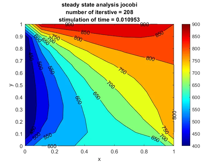
For Jacobi method
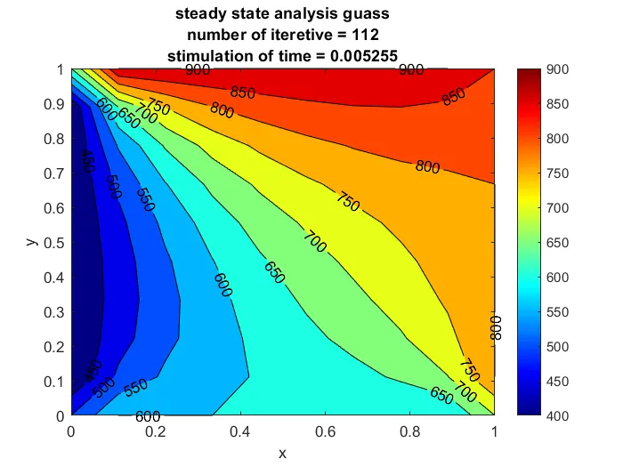
For gauss sidels method
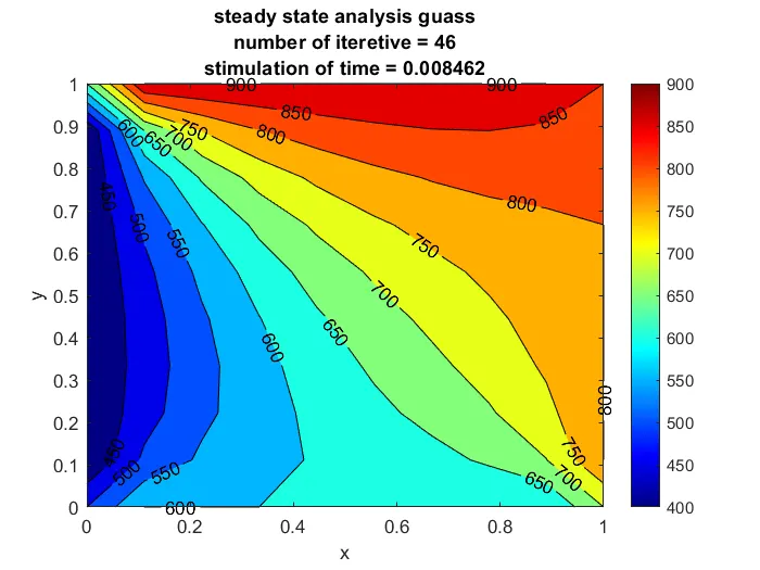
For SOR Method :
Conlusion :
we plotted a graphs for by that we can clearly say that SOR method given result with less iteratvie than the other methods
2. Transient Analysis : In transient analysis we have two following schemes :
1. implisit scheme
2. explisit scheme
Matlab code :
% Writing the program for solving the steady state analysis of 2D heat
%Conduction equation
clear all
close all
clc
%Defining the inputs as given in the question
%length of domain
L=1;
nx = 10;
ny = 10;
nt = 300;
x = linspace(0,1,nx);
y = linspace(0,1,ny);
%defining the distance between the nodes
dx = x(2)-x(1);
dy = y(2)-y(1);
%defining the boundary conditions
t = 300*ones(nx,ny);
t(1,:) = 600;
t(nx,:) = 900;
t(:,ny) = 800;
t(:,1) = 400;
% defining the corners points of the temperature
t(1,1) = 500;
t(1,ny) = 700;
t(nx,1) = 650;
t(nx, ny) = 850;
%defining the old value
dt = 0.01;
t_old = t;
alpha = 0.3;
tprev_dt = t_old;
%defining the error
error = 100;
%defining the tolerance as given in the question
tol = 1e-4;
%defining the constant value which we get in the wquation
k_1 = alpha*(dt/(dx^2));
k_2 = alpha*(dt/(dy^2));
%defining the iterative value
method = input('iterative_method = ');
%jocobiean method of solving the equation
if(method == 1)
tic;
jocobi = 1;
for k = 1:nt
while(error>tol)
for i = 2:nx-1
for j = 2:ny-1
term_1 = (1+(2*k_1)+2*k_2)^-1;
term_2 = t_old(i,j);
term_3 = t(i-1,j)+t(i+1,j);
term_4 = t(i,j-1)+t(i,j+1);
t(i,j) = ((term_1)*(term_2))+((k_1)*(term_1)*(term_3))+((k_2)*(term_1)*(term_4));
end
end
error = max(max(abs(t-t_old)));
t_old=t;
jocobi = jocobi+1;
end
tprev_dt = t;
end
time_step = toc;
%plotting the figure
figure(1)
contourf(x,y,t, 'ShowText','on')
colormap("jet")
colorbar
xlabel('x')
ylabel('y')
text_1 = sprintf('iterative_method = %d',jocobi);
text_2 = sprintf('stimulation of time = %f',time_step);
title({'unsteady state analysis using explisit';text_1;text_2});
end
% gausian method of solving the equation
if (method == 2)
tic;
guass=1;
for k = 1:nt
while(error>tol)
for i = 2:nx-1
for j = 2:ny-1
term_1 = (1+(2*k_1)+2*k_2)^-1;
term_2 = t(i,j);
term_3 = t(i-1,j)+t(i+1,j);
term_4 = t(i,j-1)+t(i,j+1);
t(i,j) = ((term_1)*(term_2))+((k_1)*(term_1)*(term_3))+((k_2)*(term_1)*(term_4));
end
end
error=max(max(abs(t-t_old)));
t_old=t;
guass=guass+1;
end
tprev_dt = t;
end
time_step = toc;
% plotting the figure
figure(2)
contourf(x,y,t,'ShowText','on')
colormap("jet")
colorbar
xlabel('x')
ylabel('y')
text_1 = sprintf('iteretive_method = %d',guass);
text_2 = sprintf('simulation of time = %f',time_step);
title({'unsteady state analysis using implisit';text_1;text_2});
end
%solving using the succesive over relaxing method
omega = 1.2;
if (method == 3)
tic;
sor=1;
for k=1:nt
while (error>tol)
for i = 2:nx-1
for j = 2:ny-1
term_1 = (1+(2*k_1)+2*k_2)^-1;
term_2 = t(i,j);
term_3 = t(i-1,j)+t(i+1,j);
term_4 = t(i,j-1)+t(i,j+1);
t(i,j) = ((((term_1)*(term_2))*(1-omega))+((omega)*((term_1)*(term_2))+((k_1)*(term_1)*(term_3))+((k_2)*(term_1)*(term_4))));
end
end
error=max(max(abs(t-t_old)));
t_old=t;
sor=sor+1;
end
time_step = toc;
end
% plotting the figure
figure(3)
contourf(x,y,t,'ShowText','on')
colormap("jet")
colorbar
xlabel('x')
ylabel('y')
text_1 = sprintf('number of iteretive = %d',sor);
text_2 = sprintf('simulation of time = %f',time_step);
title({'unsteady state analysis using implisit';text_1;text_2});
end
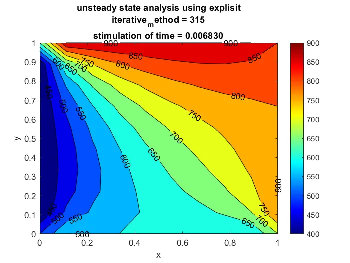
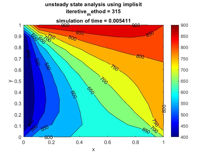
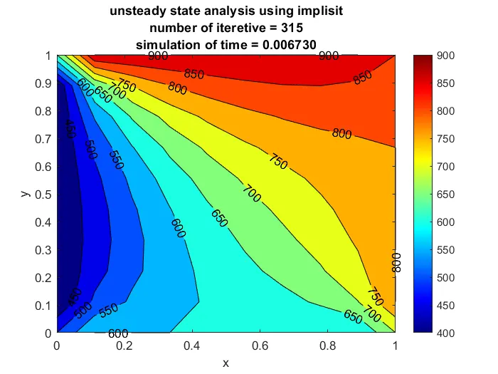
Outputs :
 \
\