Challenge

Week 3 - Solving second order ODEs

SSandeep Kolaparthi5 Apr 2022

Aim : To solve second order diffrential equation using Matlab.

Objectives :

1. Write a program in Matlab\Octave that will simulate the pendulum motion.

Your objective is to write a program that solves the following ODE. This ODE represents the equation of motion of a simple pendulum with damping

In the above equation,

g = gravity in m/s2,

L = length of the pendulum in m,

m = mass of the ball in kg,

b=damping coefficient.

2. Simulate the motion between 0-20 sec, for angular displacement=0,angular velocity=3 rad/sec at time t=0.

Write a program in Matlab\Octave that will simulate the pendulum motion, just like the one shown in the start of this challenge.

use,

L=1 metre,

m=1 kg,

b=0.05.

g=9.81 m/s2.

Theory :

A pendulum is a body suspended from a fixed point so that it can swing back and forth under the influence of gravity. The time interval of a pendulum's complete back-and-forth movement is constant. When a pendulum is displaced sideways from its resting, equilibrium position, it is subject to a restoring force due to gravity that will accelerate it back toward the equilibrium position. When released, the restoring force acting on the pendulum's mass causes it to osciliate about the equilibrium position, swinging back and forth. The time for one complete cycle, a left swing and a right swing, is called the period. The period depends on the length of the pendulum and also to a slight degree on the amplitude the width of the pendulum's swing.

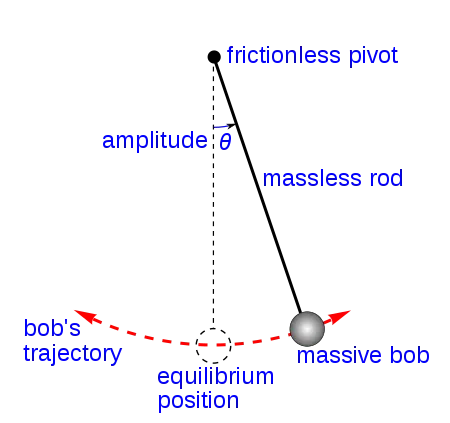
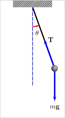
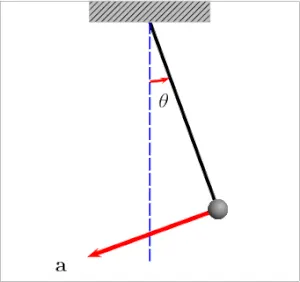
The point from which bob is suspended is known as part of suspension. Weight of the bob acts vertically downwards and the tesnsion acts vertically upwards. So the bob comes under equilibrium position and the bob starts osciliating if even smaller external force is applied.

Procedure / Explanation :

Governing Equation of second order ODE

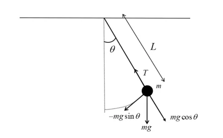
θ is the angle made by movable link with vertical axis

L is the length of movable rod

m is the mass of the bob, b is the damping coeffieicent od the system.

-------------> second order ODE------(1)

To solve this ODE we need to reduce the order of equation in to lower order

let θ = θ1

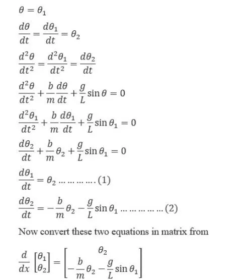
Now we derived (1) and (2) equation,

Given details,

simulate the motion between 0-20 sec

for angular displacement = 0

at Time = 0

angular velocity = 3 rad/sec

L =1 m

m = 1 kg

b=0.05.

g=9.81 m/s2.

assign the given parameters as variables in the code. The time span of the pendulum is set by usinglinspace command, theta value is given as a column matrix.
we have write ode45 function and name the function as ode_func as same as the name in the function
Plot a graph corrsponding to time and velocity, put a legend to identify the each values of the graph.
for accurate simulation of the simple pendulum corresponding to second order ode with damping we need to use the looping statements, here for loop is used to create.
The pendulum has fixed cocordinates mentioned as x0,y0 and x1y1 are the second coordinates
marker command is used for making motion of the bon for the pendulum, the axis is fixed using axis command
The countour command is used to make the value changes in each for loop. the videowiter command is used to create the video file.
Save the video and closw the video by giving save video_file and close video_file commands and uploaded the video in youtube.

Code used :

Programming language : Matlab

1. code function of ode45 for main program -

function [dtheta_dt] = ode_func(t,theta,b,g,l,m)

theta1 = theta(1)

theta2 = theta(2)

dtheta1_dt = theta2;

dtheta2_dt = -(b/m)*theta2 - (g/l)*sin(theta1);

dtheta_dt = [dtheta1_dt; dtheta2_dt];

end

2. Main program

clear all

close all

clc

% solving the second order ode and show the animation

% Damping coefficient

b = 0.05;

%length of pendulum

l = 1;

%mass of bob in kg

m = 1

% gravaity in m/s^2

g = 9.81

% Initial condition

theta_0 = [0;3]

% Time points

t_span = linspace(0,20,500)

% solve ode

[t,results] = ode45(@(t,theta) ode_func(t, theta, b,g,l,m),t_span, theta_0);

figure (1)

plot(t,results(:,1))
hold on
plot(t,results(:,2))
ylabel('velocity')
xlabel('time')
legend('displacement', 'angular velocity')
grid on
hold off

displacement = results(:,1)

velocity = results(:,2)

ct=1;

for i = 1:length(results(:,1))

title('motion of pendulum')

%fixed coordinates of one end of simple pendulum

x0 = 0;

y0 = 0;

%moving coordinates of the bob

x1 = 1*sin(results(i,1));

y1 = -1*cos(results(i,1));

figure(2)

plot([-0.5 0.5],[0 0],'lineWidth',2,'Color','black')
hold on
plot([0 0],[-1.5 0.5],'LineStyle','--','Color','black')
plot([x0 x1],[y0 y1],'LineWidth',1,'Color','b')
plot(x0, y0,'o','MarkerSize',4,'MarkerFaceColor',[0.6 0.6 0.6]);
plot(x1, y1,'o','MarkerSize',20,'MarkerFaceColor','r')
axis([-1.5 1.5 -1.5 0.5])
pause(0.01)
M(ct) = getframe(gcf);
ct = ct+1;
hold off

end

movie(M)

video_file = VideoWriter('pendulum challenge.avi','Uncompressed AVI')

open(video_file)

writeVideo(video_file,M)

close(video_file)

Results :

1. graph represents the pendulum motion :

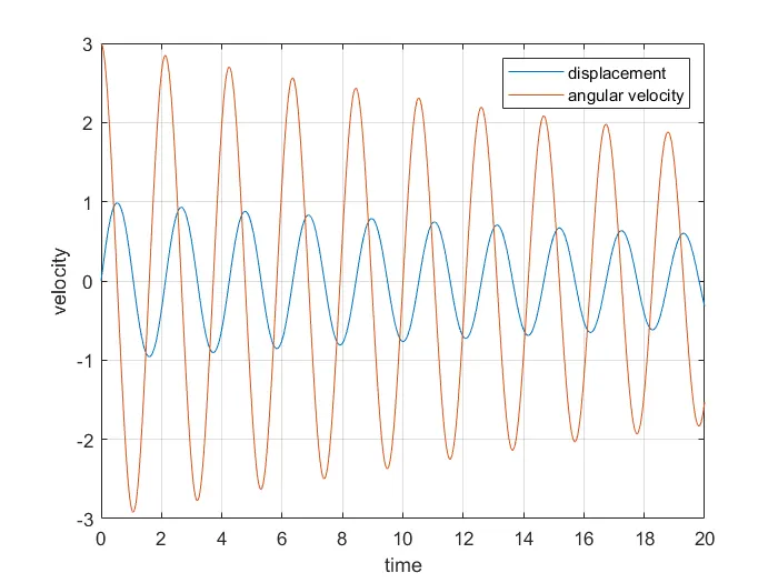
2. Simulated the motion between for given angular displacement and angular velocity

Animation link of the simple pendulum.

https://youtu.be/VhbTW_P9kIU

Errors occured :

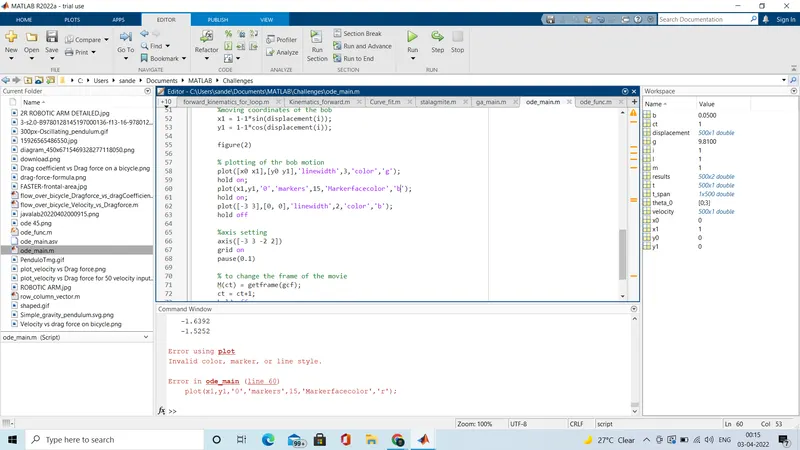
error occured while plotting the bob motion, markersize, linestyle, markerface color inputs not given propely. It is corrected by checking inputs properly after several trails by executing the program.

References :

1. https://en.wikipedia.org/wiki/Pendulum

2. https://study.com/academy/answer/draw-a-free-body-diagram-of-a-pendulum-while-in-motion-calculate-the-period-t-for-a-pendulum-of-length-l-and-mass-m-does-the-period-depend-on-the-mass-of-the-pendulum-explain.html

Week 3 - Solving second order ODEs

Ship work like this
in your own course.

Talk to a career counsellor

Ship work like thisin your own course.

Talk to a career counsellor

Ship work like this
in your own course.