Week 4.1 - Genetic Algorithm
Aim :
- Write a code in MATLAB to optimise the stalagmite function and find the global maxima of the function.
- To explain the concept of genetic algorithm in our own words and also explain the syntax for ga in MATLAB in our report.
- Plot graphs for all 3 studies and for F maximum vs no. of iterations. Title and axes labels are a must, legends could be shown if necessary.
Theory :
Genetic Algorithm - The genetic algorithm is a method for solving both constrained and unconstrained optimization problems that is based on natural selection, the process that drives biological evolution. The genetic algorithm repeatedly modifies a population of individual solutions.
A genetic algorithm is a search heuristic that is inspired by Charles Darwin’s theory of natural evolution. This algorithm reflects the process of natural selection where the fittest individuals are selected for reproduction in order to produce offspring of the next generation.
Example code :
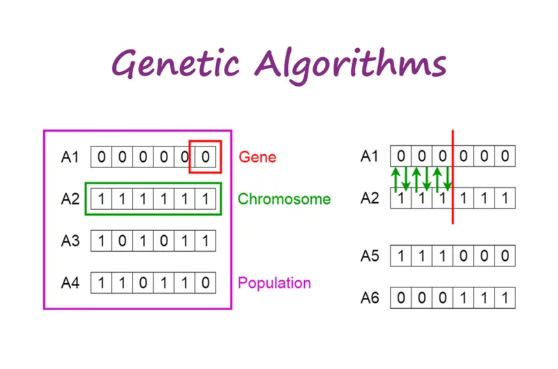
Notion of natural sellection :
The process of natural selection starts with the selection of fittest individuals from a population. They produce offspring which inherit the characteristics of the parents and will be added to the next generation. If parents have better fitness, their offspring will be better than parents and have a better chance at surviving. This process keeps on iterating and at the end, a generation with the fittest individuals will be found.
This notion can be applied for a search problem. We consider a set of solutions for a problem and select the set of best ones out of them.
Five phases are considered in a genetic algorithm.
- Initial population
- Fitness function
- Selection
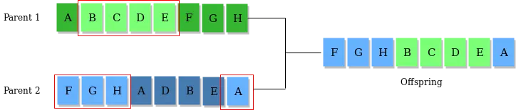
- Crossover
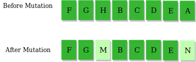
- Mutation
Genetic algorithms are commonly used to generate high-quality solutions to optimization and search problems by relying on biologically inspired operators such as mutation, crossover and selection.
Search space :

Cross operator :
Mutation operator :
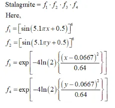
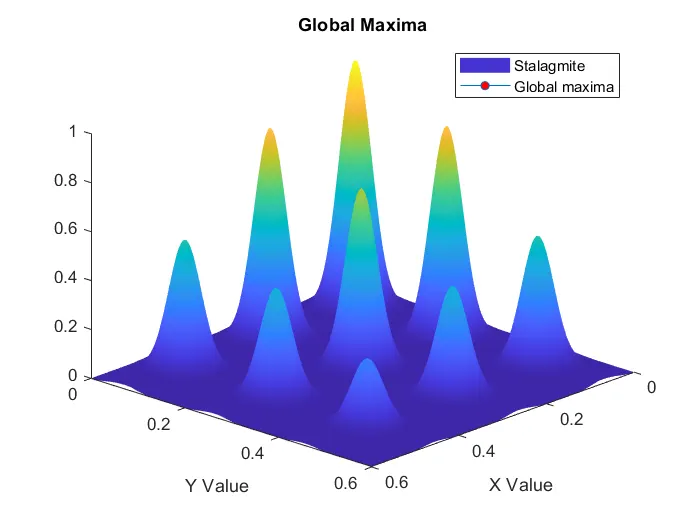
Defining the stalagmite function code :
Explanation of the code :
Procudure for obtaining stalagmite function values :
- get_stalagmite function accepts the x and y values as input
- use meshgrid command to generate mesh of x and y
- use for loop to run through the whole mesh and access all the defined grid points
- The x and y value at each grid point is paased to stalagmite function and function value is obtained
Procedure for running genetic algorithm to obtain global maxima :
- Generate the equispaced values on x and y axis using linspace command.
- Use values as input to get_stalagmite function to obtain the stalagmite values at all grid points.
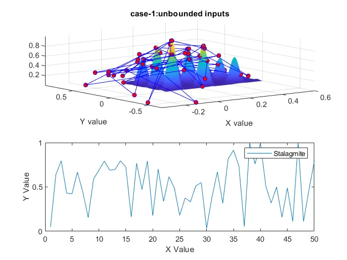
- In the first study, only the fitness function and number of variables are passed as input in 'ga' function. Hence this study case is unbounded in nature.
- All the fit coordinates are stored in inputs and segregated in to x out and y out variables. f out stores the global and local maxima.
- The results are plotted, 'srfc' command is used to plot contours under the surface plot. 'shading' command is used to remove the grid lines on the surface and 'interp' command is used for interpolation, to smoothen the curve. 'plot3' command is used to plot the values in 3-dimensions. The results obtained from 'ga' is used to mark the coordinates in the 3D space which represent the global and local maxima.
- Then 'plot' command is used to plot the optimized function values againsts every iteration. 'subplot' command is used ti divide the figure windows to it in various plots. In this case, figure window is divided into 2 rows and 1 column.
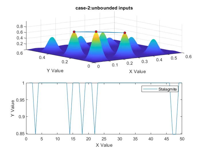
- In the second study, the lower bounds and upper bounds are also passed as input arguments in 'ga'.
- since there are no linear inequalities, empty matrices[] are passed in the corresponding position within 'ga'.
- similarly, the same plots are generated with better results.
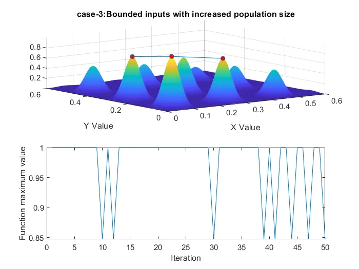
- In the third study, the population size is defined additionally.'options' is of structured data type, which is used to create population size. Whenever the input variables for fitness function is 2, then population size is set to default. This value is increased to obtain better output.
- Again the similar plots are generated.
Programming lanuguage : MATLAB
Code used in matlab :
clear all
close all
clc
% defining our search space
x = linspace(0,0.6,150);
y = linspace(0,0.6,150);
num_cases = 50;
% creating 2-dimensional grid
[x, y] = meshgrid(x,y);
% calculating the fitting function
for i = 1:length(x)
for j = 1:length(y)
input(1) = x(i,j);
input(2) = y(i,j);
f(i,j) = stalagmite_func1(input);
end
end
figure(1)
surfc(x,y,-f)
xlabel('X Value')
ylabel('Y Value')
zlabel('F value')
shading interp;
title('Global Maxima')
legend('Stalagmite','Global Maxima') output :
% study_1 statistical behaviour
iteration = 50;
tic
for i = 1:iteration
[input, fopt(i)] = ga(@stalagmite_func1,2);
xopt(i) = input(1);
yopt(i) = input(2);
end
study1_time = toc;
figure(2)
subplot(2,1,1)
surfc(x,y,-f)
xlabel('X value')
ylabel('Y value')
shading interp
hold on
plot3(xopt,yopt,-fopt,'color','b','marker','o','markersize',5,'MarkerFaceColor','r');
title('case-1:unbounded inputs')
subplot(2,1,2)
plot(-fopt)
xlabel('X Value')
ylabel('Y Value')
legend('Stalagmite','Global Maxima')output : study 1
% study_2 Staistical behaviour with upper and lower bounds
tic
for i = 1:iteration
[input2, fopt(i)] = ga(@stalagmite_func1,2,[],[],[],[],[0;0],[0.4;0.4]);
xopt(i) = input2(1);
yopt(i) = input2(2);
end
study_2_time = toc;
figure(3)
subplot(2,1,1)
surfc(x,y,-f);
xlabel('X Value')
ylabel('Y Value')
shading interp
hold on
plot3(xopt,yopt,-fopt,'marker','o','markersize',5,'MarkerFaceColor','r');
title('case-2:unbounded inputs')
subplot(2,1,2)
plot(-fopt)
xlabel('X Value')
ylabel('Y Value')
legend('Stalagmite','Global Maxima')ouput : study 2
%study_3 statistical behaviour with bounded inputs and icreased population
options = optimoptions('ga');
options = optimoptions(options, 'PopulationSize',100);
tic
for i = 1:iteration
[input3, fopt(i)] = ga(@stalagmite_func1,2,[],[],[],[],[0;0],[0.4;0.4]);
xopt(i) = input3(1);
yopt(i) = input3(2);
end
study_3_time = toc;
figure(4)
subplot(2,1,1)
surfc(x,y,-f)
shading interp
xlabel('X Value')
ylabel('Y Value')
hold on
plot3(xopt,yopt,-fopt,'marker','o','markersize',5,'MarkerFaceColor','r');
title('case-3:Bounded inputs with increased population size')
subplot(2,1,2)
plot(-fopt)
xlabel('Iteration')
ylabel('Function maximum value')
output : study 3
References :