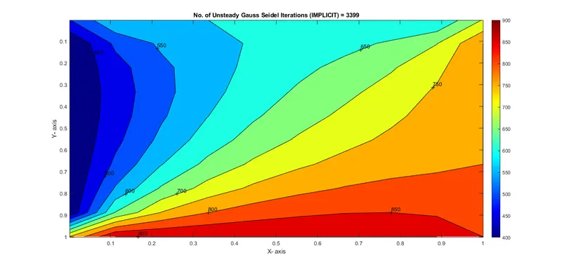
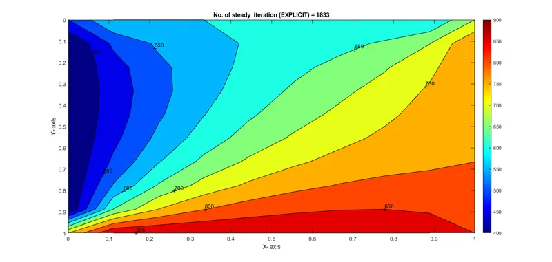
1. Steady state analysis & Transient State Analysis
Solve the 2D heat conduction equation by using the point iterative techniques that were taught in the class. The Boundary conditions for the problem are as follows;
Top Boundary = 600 K
Bottom Boundary = 900 K
Left Boundary = 400 K
Right Boundary = 800 K
You will implement the following methods for solving implicit equations.
1. Jacobi
2. Gauss-seidel
3. Successive over-relaxation
Your absolute error criteria is 1e-4
Theory:-
The heat equation is a partial differentional equation that describes how the distribution of some quantity (such as heat) evolves over time in a solid medium, as it spontaneously flow places where it is higher towards places where it is lower.
for a function u(x,y,z,t) of three spatial variables (x,y,z) and time vriable t, the heat equation is
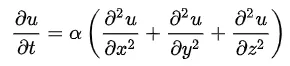
where,
alpha a is real coefficient the diffusivity of the medium.
Type of Heat Condution schemes
- Steady state Condition
- Unsteady/Transient State condtion
Unsteady state condtions are a precursor to steady state condition. no system exists initiallu under steady state conditions. some tiem must be pass after heat transfer is initialed before the system reaches steady state. during that period of transition the system is under unsteady state condition.
Governing Equations:-
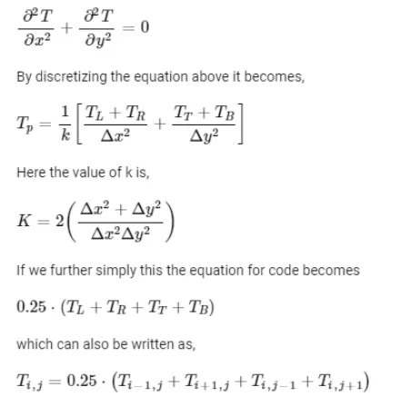
In order to slove 2D heat conduction problem the governing equation for respective condition with respect to cartesian coordinates should be discretized to enter that in a code which is given by main program below.
MAIN PROGRAMS:-
below there is a sequence of seven indivdual program, stating with implicit scheme of steady & unsteady state conditions for three iterative Jacobi Gauss-seidel Successive over-relaxation .
Implicit Scheme-steady-state condition
steady state equations
In steady state condition the amount of heat entering any region of an obejct is equal to the amount of heat coming out (if were not so the temp. would be rising of falling as thermal energy was tapped in a region)
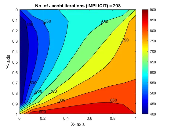
Jacobi Iteration program
close all
clear all
clc
%Solving the Steady 2D heat conduction (Jacobi Method)
% Input Parameters
%number of grid points
nx = 10;
ny = nx;
x = linspace(0,1,nx);
y = linspace(0,1,ny);
dx = x(2)-x(1);
dy = dx;
%absulate error criteeria > tolerance
error = 9e9;
tolerance = 1e-4;
%define Boundary condtions
T_L = 400;
T_T = 600;
T_R = 800;
T_B = 900;
T = 300*ones(nx,ny);
T(2:ny-1, 1)=T_L;
T(2:ny-1, nx)=T_R;
T(1, 2:nx-1)=T_T;
T(ny, 2:nx-1)=T_B;
%calculating Average temperature at corners
T(1,1) = (T_T+T_L)/2;
T(nx,ny) = (T_R+T_B)/2;
T(1,ny) = (T_T+T_R)/2;
T(nx,1) = (T_T+T_B)/2;
%Assigning orignal values to T
T_intial = T;
T_old = T;
% calculation of 2D steady heat condutions Equations by Jacobi method
iterative_solver = 1;
if iterative_solver == 1
jacobi_iteration = 1;
while(error > tolerance)
for i = 2:nx-1
for j = 2:ny-1
T(i,j) = 0.25*(T_old(i-1,j)+T_old(i+1,j)+T_old(i,j-1)+T_old(i,j+1));
end
end
error = max(max(abs(T_old - T)));
T_old = T;
jacobi_iteration = jacobi_iteration+1;
end
end
%plotting
figure(1)
contourf(x,y,T)
clabel(contourf(x,y,T))
colorbar
colormap(jet)
set(gca, 'ydir', 'reverse')
xlabel('X- axis')
ylabel('Y- axis')
title(sprintf('No. of Jacobi Iterations (IMPLICIT) = %d', jacobi_iteration));
pause(0.03);
Output:-
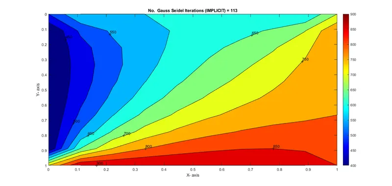
Gauss seidel-iteration program
close all
clear all
clc
%Solving the Steady 2d heat conduction (Gauss-seidel Method)
% Input Parameters
%number of grid points
nx = 10;
ny = nx;
x = linspace(0,1,nx);
y = linspace(0,1,ny);
dx = x(2)-x(1);
dy = dx;
%absulate error criteria > tolerance
error = 9e9;
tolerance = 1e-4;
%define Boundary condtions
T_L = 400;
T_T = 600;
T_R = 800;
T_B = 900;
T = 300*ones(nx,ny);
T(2:ny-1, 1)=T_L;
T(2:ny-1, nx)=T_R;
T(1, 2:nx-1)=T_T;
T(ny, 2:nx-1)=T_B;
%calculating Average temperature at corners
T(1,1) = (T_T+T_L)/2;
T(nx,ny) = (T_R+T_B)/2;
T(1,ny) = (T_T+T_R)/2;
T(nx,1) = (T_T+T_B)/2;
%Assigning orignal values to T
T_intial = T;
T_old = T;
% calculation of 2D steady heat condutions Equations Gauss-seidel Method
iterative_solver = 2;
if iterative_solver == 2
Gauss_seidel_iteration = 2;
while(error > tolerance)
for i = 2:nx-1
for j = 2:ny-1
T(i,j) = 0.25*(T(i-1,j)+T_old(i+1,j)+T(i,j-1)+T_old(i,j+1));
end
end
error = max(max(abs(T_old - T)));
T_old = T;
Gauss_seidel_iteration = Gauss_seidel_iteration+1;
end
end
%plotting
figure(1)
contourf(x,y,T)
clabel(contourf(x,y,T))
colorbar
colormap(jet)
set(gca, 'ydir', 'reverse')
xlabel('X- axis')
ylabel('Y- axis')
title(sprintf('No. Gauss Seidel Iterations (IMPLICIT) = %d',Gauss_seidel_iteration));
pause(0.03);
Output:-
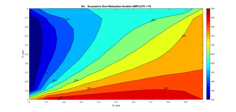
Successive over-relaxation method:-
close all
clear all
clc
%Solving the Steady 2d heat conduction (Successive over-relaxation Method)
% Input Parameters
%number of grid points
nx = 10;
ny = nx;
x = linspace(0,1,nx);
y = linspace(0,1,ny);
dx = x(2)-x(1);
dy = dx;
%absulate error criteria > tolerance
error = 9e9;
tolerance = 1e-4;
omega = 1.2;
%define Boundary condtions
T_L = 400;
T_T = 600;
T_R = 800;
T_B = 900;
T = 300*ones(nx,ny);
T(2:ny-1, 1)=T_L;
T(2:ny-1, nx)=T_R;
T(1, 2:nx-1)=T_T;
T(ny, 2:nx-1)=T_B;
%calculating Average temperature at corners
T(1,1) = (T_T+T_L)/2;
T(nx,ny) = (T_R+T_B)/2;
T(1,ny) = (T_T+T_R)/2;
T(nx,1) = (T_T+T_B)/2;
%Assigning orignal values to T
T_intial = T;
T_old = T;
% calculation of 2D steady heat condutions Equations by Successive over relaxation method
iterative_solver = 3;
if iterative_solver == 3
Successive_Over_Relaxation_iteration = 1;
while(error > tolerance)
for i = 2:nx-1
for j = 2:ny-1
T(i,j) = omega*(0.25*(T(i-1,j)+T_old(i+1,j)+T(i,j-1)+T_old(i,j+1)))+(1-omega)*T_old(i,j);
end
end
error = max(max(abs(T_old - T)));
T_old = T;
Successive_Over_Relaxation_iteration = Successive_Over_Relaxation_iteration + 1;
end
end
%plotting
figure(1)
contourf(x,y,T)
clabel(contourf(x,y,T))
colorbar
colormap(jet)
set(gca, 'ydir', 'reverse')
xlabel('X- axis')
ylabel('Y- axis')
title(sprintf('No.Successive Over-Relaxation iteration (IMPLICIT) = %d', Successive_Over_Relaxation_iteration ));
pause(0.03);
outputs:-
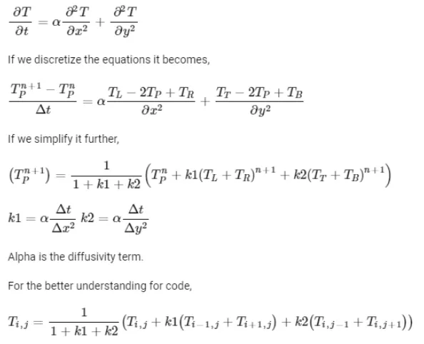
Implicit Schame Unsteady/Transient State condtion:
Unsteady/Transient State equation disretizations:-
unsteady state situations appear after an imposed change in temprature at a boundary as well as inside of an object an a result of a new source or sink of heat suddenly introduced within an object, cousing temperatures near the source or sink to change in time.
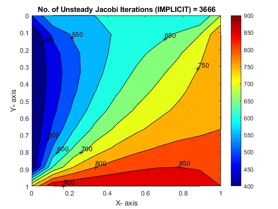
Unsteady Jacobi Iteration program
close all
clear all
clc
%Solving the Unsteady 2D heat conduction Jacobi Method (IMPLICIT SCHEME)
% Input Parameters
%number of grid points
nx = 10;
ny = nx;
nt = 1400;
x = linspace(0,1,nx);
y = linspace(0,1,ny);
dx = x(2)-x(1);
dy = dx;
%absulate error criteeria > tolerance
error = 9e9;
tolerance = 1e-4;
dt = 1e-3;
%define Boundary condtions
T_L = 400;
T_T = 600;
T_R = 800;
T_B = 900;
T = 300*ones(nx,ny);
T(2:ny-1, 1)=T_L;
T(2:ny-1, nx)=T_R;
T(1, 2:nx-1)=T_T;
T(ny, 2:nx-1)=T_B;
%calculating Average temperature at corners
T(1,1) = (T_T+T_L)/2;
T(nx,ny) = (T_R+T_B)/2;
T(1,ny) = (T_T+T_R)/2;
T(nx,1) = (T_T+T_B)/2;
%Assigning orignal values to Temprature
T_old = T;
T_intial = T;
T_prvious_dt = T_old;
% calculate the 2D steady heat condution equation
k1 = 1.4*(dt/(dx^2));
k2 = 1.4*(dt/(dy^2));
% calculation of 2D unsteady heat condutions Equations by Jacobi method
jacobi_iteration = 1;
for k = 1:nt
error = 9e9;
while(error > tolerance)
for i = 2:nx - 1
for j = 2:ny - 1
term_1 = (1 + (2*k1) + (2*k2))^-1;
term_2 = k1*term_1;
term_3 = k2*term_1;
H = (T_old(i-1,j)) + (T_old(i+1,j));
V = (T_old(i,j+1)) + (T_old(i,j-1));
T(i,j) = (T_prvious_dt(i,j)*term_1) + (H*term_2) + (V*term_3);
end
end
error = max(max(abs(T_old - T)));
T_old = T;
jacobi_iteration = jacobi_iteration + 1;
end
T_prvious_dt=T;
end
%plotting
figure(1)
contourf(x,y,T)
clabel(contourf(x,y,T))
colorbar
colormap(jet)
set(gca, 'ydir', 'reverse')
xlabel('X- axis')
ylabel('Y- axis')
title(sprintf('No. of Unsteady Jacobi Iterations (IMPLICIT) = %d', jacobi_iteration));
pause(0.03);
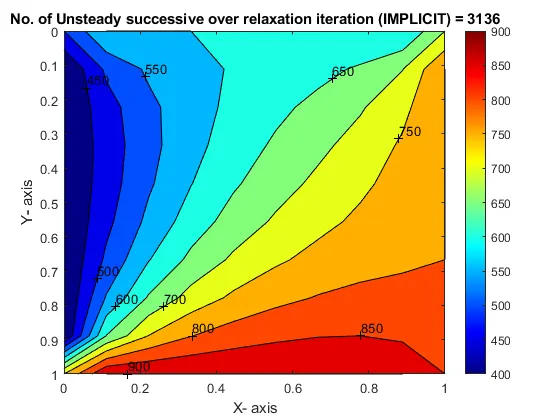
Output:-
Unsteady Gauss seidel-iteration program
close all
clear all
clc
%Solving the unsteady 2d heat conduction (Gauss-seidel Method)
% Input Parameters
%number of grid points
nx = 10;
ny = nx;
nt = 1400;
x = linspace(0,1,nx);
y = linspace(0,1,ny);
dx = x(2)-x(1);
dy = dx;
%absulate error criteria > tolerance
error = 9e9;
tolerance = 1e-4;
dt = 1e-3
%define Boundary condtions
T_L = 400;
T_T = 600;
T_R = 800;
T_B = 900;
T = 300*ones(nx,ny);
T(2:ny - 1, 1) = T_L;
T(2:ny - 1, nx) = T_R;
T(1, 2:nx - 1) = T_T;
T(ny, 2:nx - 1) = T_B;
%calculating Average temperature at corners
T(1,1) = (T_T+T_L)/2;
T(nx,ny) = (T_R+T_B)/2;
T(1,ny) = (T_T+T_R)/2;
T(nx,1) = (T_T+T_B)/2;
%Assigning orignal values to T
T_old = T;
T_intial = T;
T_prvious_dt = T_old;
% calculation of 2D unsteady heat condutions Equations by Jacobi method
k1 = 1.4*(dt/(dx^2));
k2 = 1.4*(dt/(dy^2));
Gauss_seidel_iteration = 2;
for k = 1:nt
error = 9e9;
while(error > tolerance)
for i = 2:nx - 1
for j = 2:ny - 1
term_1 = 1/(1+(2*k1)+(2*k2));
term_2 = k1*term_1;
term_3 = k2*term_1;
H = (T(i-1,j)) + (T_old(i+1,j));
V = (T(i,j+1)) + (T_old(i,j-1));
T(i,j) = (T_prvious_dt(i,j)*term_1) + (H*term_2) + (V*term_3);
end
end
error = max(max(abs(T_old - T)));
T_old = T;
Gauss_seidel_iteration = Gauss_seidel_iteration+1;
end
T_prvious_dt = T_old;
end
%plotting
figure(1)
contourf(x,y,T)
clabel(contourf(x,y,T))
colorbar
colormap(jet)
set(gca, 'ydir', 'reverse')
xlabel('X- axis')
ylabel('Y- axis')
title(sprintf('No. of Unsteady Gauss Seidel Iterations (IMPLICIT) = %d', Gauss_seidel_iteration));
pause(0.03);
Output:-
Successive over-relaxation method program:-
close all
clear all
clc
%Solving the unsteady 2d heat conduction successive over relaxations method (impicit)
% Input Parameters
%number of grid points
nx = 10;
ny = nx;
nt = 1400;
x = linspace(0,1,nx);
y = linspace(0,1,ny);
dx = x(2)-x(1);
dy = dx;
%absulate error criteria > tolerance
error = 9e9;
tolerance = 1e-4;
dt = 1e-3;
omega = 1.1;
%define Boundary condtions
T_L = 400;
T_T = 600;
T_R = 800;
T_B = 900;
T = 300*ones(nx,ny);
T(2:ny - 1, 1) = T_L;
T(2:ny - 1, nx) = T_R;
T(1, 2:nx - 1) = T_T;
T(ny, 2:nx - 1) = T_B;
%calculating Average temperature at corners
T(1,1) = (T_T+T_L)/2;
T(nx,ny) = (T_R+T_B)/2;
T(1,ny) = (T_T+T_R)/2;
T(nx,1) = (T_T+T_B)/2;
%Assigning orignal values to T
T_old = T;
T_intial = T;
T_end = T;
% calculation of 2D unsteady heat condutions Equations by successive over relaxation method
k1 = 1.4*(dt/(dx^2));
k2 = 1.4*(dt/(dy^2));
successive_over_relaxation_iteration = 1;
for k = 1:nt
error = 9e9;
while(error > tolerance)
for i = 2:nx - 1
for j = 2:ny - 1
term_1 = 1/(1+(2*k1)+(2*k2));
term_2 = k1*term_1;
term_3 = k2*term_1;
H = (T(i-1,j)) + (T_old(i+1,j));
V = (T(i,j+1)) + (T_old(i,j-1));
T(i,j) = (T_intial(i,j)*term_1) + (H*term_2) + (V*term_3);
T_end(i,j) = ((1-omega)*T_old(i,j)) + (T(i,j)*omega);
end
end
error = max(max(abs(T_old - T)));
T_old = T_end;
successive_over_relaxation_iteration = successive_over_relaxation_iteration + 1;
end
T_intial= T_end;
end
%plotting
figure(1)
contourf(x,y,T)
clabel(contourf(x,y,T))
colorbar
colormap(jet)
set(gca, 'ydir', 'reverse')
xlabel('X- axis')
ylabel('Y- axis')
title(sprintf('No. of Unsteady successive over relaxation iteration (IMPLICIT) = %d', successive_over_relaxation_iteration ));
pause(0.03);
EXPICIT schame Unsteady/Transient State condition program
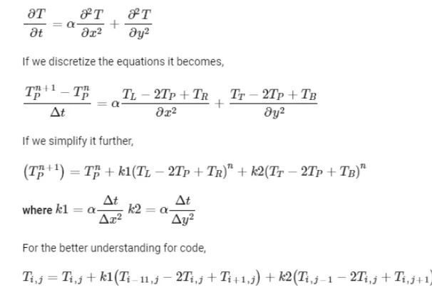
Unsteady/Transient State condition discritization(EXPICIT)
EXPLICIT Scheme program
close all
clear all
clc
%Solving the unsteady state 2d heat conduction (EXOLICIT SCHEME)
% Input Parameters
%number of grid points
nx = 10;
ny = nx;
nt = 1400;
x = linspace(0,1,nx);
y = linspace(0,1,ny);
dx = x(2)-x(1);
dy = dx;
%absulate error criteria > tolerance
error = 9e9;
tolerance = 1e-4;
dt = 1e-3;
omega = 1.1;
%define Boundary condtions
T_L = 400;
T_T = 600;
T_R = 800;
T_B = 900;
T = 300*ones(nx,ny);
T(2:ny - 1, 1) = T_L;
T(2:ny - 1, nx) = T_R;
T(1, 2:nx - 1) = T_T;
T(ny, 2:nx - 1) = T_B;
%calculating Average temperature at corners
T(1,1) = (T_T+T_L)/2;
T(nx,ny) = (T_R+T_B)/2;
T(1,ny) = (T_T+T_R)/2;
T(nx,1) = (T_T+T_B)/2;
%Assigning orignal values to T
T_old = T;
T_intial = T;
% calculation of 2D unsteady heat condutions Equations
iterative_solver = 1;
k1 = 1.4*(dt/(dx^2));
k2 = 1.4*(dt/(dy^2));
if iterative_solver == 1
Steady_Explicit = 1;
for k = 1:nt
error = 1;
while(error > tolerance)
for i = 2:nx - 1
for j = 2:ny - 1
term_1 = T_old(i,j);
term_2 = k1*(T_old(i+1,j) - 2*T_old(i,j)+(T_old(i-1,j)));
term_3 = k2*(T_old(i,j+1) - 2*T_old(i,j)+(T_old(i,j-1)));
T(i,j) = term_1+term_2+term_3;
end
end
error = max(max(abs(T_old - T)));
T_old = T;
Steady_Explicit = Steady_Explicit + 1;
end
end
end
%plotting
figure(1)
contourf(x,y,T)
clabel(contourf(x,y,T))
colorbar
colormap(jet)
set(gca, 'ydir', 'reverse')
xlabel('X- axis')
ylabel('Y- axis')
title(sprintf('No. of steady iteration (EXPLICIT) = %d', Steady_Explicit ));
pause(0.03);
Outputs:-
Conclusion:-
- jacobi>gauss-seidel>successive over-relaxation according to the no of iteration, we can canclude that method &scheme.
- when comparing steady state and unsteady state it isd proven that steady state is the most successful one as it takes least number of iterations and least time to compare.
- SoR iteration method is most effective method as it took least No. of iterations for coverging solutions in both the schemes (EXPICIT & IMPICIT) compared to jacobi and gauss seidel method.