Week 3.5 - Deriving 4th order approximation of a 2nd order derivative using Taylor Table method

Aim:-Derive the following 4th order approximations of the second-order derivative.

1. Central difference

2. Skewed right-sided difference

3. Skewed left-sided differencederivative of the analytical function exp(x)*cos(x) and compare it with the 3 numerical approximations that you have derived.

Introduction:-

Taylor series is the polynomial or a function of an infinite sum of terms. Each successive term will have a larger exponent or higher degree than the preceding term.

The above Taylor series expansion is given for a real values function f(x) where f’(a), f’’(a), f’’’(a), etc., denotes the derivative of the function at point a. If the value of point ‘a’ is zero, then the Taylor series is also called the Maclaurin series.

In terms of sigma notation, the Taylor series can be written as

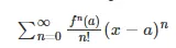
Where

f⁽ⁿ⁾ (a) = n^th derivative of

n! = factorial of n.

Formulas and Calculations

Deriving the fourth order approximation for the second order derivative using.

Central Differencing Method:-

It is refered to as central defferencing method becouse it take the values from the current point as well as both the previous (L.H.S)

and next (R.H.S) point.

here we are computing 4th order approximation at point f(i), where we take infromation from the four point surrounding f(i); that is we are going to take twof o ponts on the left f(i) and two point on the right of f(i). Let those points be f(i-2), f(i-1), f(i+1), and f(i+2) and the distance between each of them is (`(/_\\`x)`. our numerical stencil will look like show the fig.

According to given data for the central differencing

Number of node,

N = P+Q-1

where,

P = Order of derivative

Q = Order of approximation

as we are computing the 4th order approximation for 2nd order derivative we get,

N = 2+4-1

N = 5

therefore, this means that we required 5 nodes to get required accuracy.

there by formulating the hypothesis equation base on 5 nodes,

...... Equation(1)

Taylor series expansion trems:-

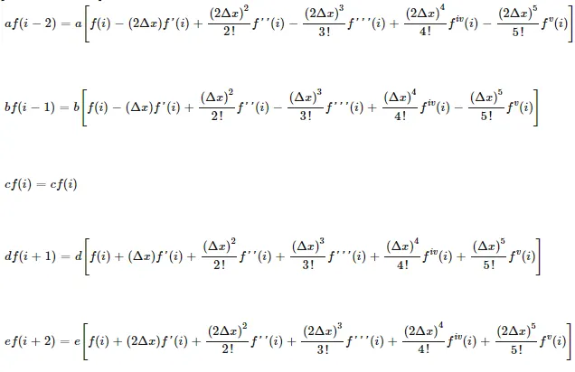
Taylor series tables:-

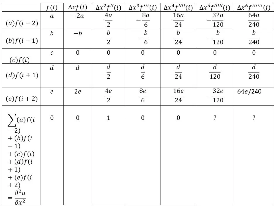
we have slove five equations and get values of coefficients (a,b,c,d,e).

We are going to from these equation by adding terms for the individual columns.

the summation of coefficients of f'(i) is equal to 1, and f(i), f'(i), f''(i), f'''(i), f''''(i), are equal to 0; becouse we want to calculate the second - order derivative , f'(i).

therefore five equation are;

a+b+c+d+e = 0 .........(i)

-2a-b+0+d+2e = 0 .........(ii)

`2a+b/2+0+d/2+2e = 1 ........(iii)

-8a/6-b/6+0+d/6+8e/6 = 0 ........(iv)

16a/24+b/24+0+d/24+16e/24 = 0 ........(v)

To get the all five equation solution in matrix form; AX=B

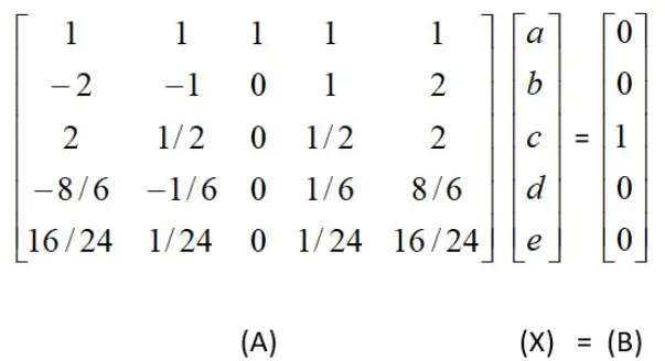
After solving the above the matrix we get value of all coefficients as;

a = -0.083333 or -1/12

b = 1.333333 or 4/3

c = -2.500000 or -5/2

d = 1.333333 or 4/3

e = 0.083333 or -1/12

here,

a = e, and b=d

there by substituting the above value in hyoithesis equation

taking L.C.M of the denominator trrms the fourth order approximation equation for second order derivative by central differecing method as follows

Skewed right-sided difference method :-

It is refered to as Skewed right-sided difference method becouse it take the values from the current point as well as both the next points(R.H.S).

to derive 4th order Skewed right-sided difference method at point f(i) of function. since we are using Skewed right-sided difference method. here we have to define five points on the right of f(i). let those points be f(i+1), f(i+2), f(i+3), f(i+4), and f(i+5) with each a sapcing of (`(/_\\`x)`.

Number of node,

N = P+Q

where,

P = Order of derivative

Q = Order of approximation

as we are computing the 4th order approximation for 2nd order derivative we get,

N = 2+4

N = 6

therefore, this means that we required 6 nodes to get required accuracy.

there by formulating the hypothesis equation base on 6 nodes,

........(2)

Taylor series expansion trems:-

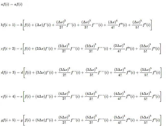
Taylor series tables:-

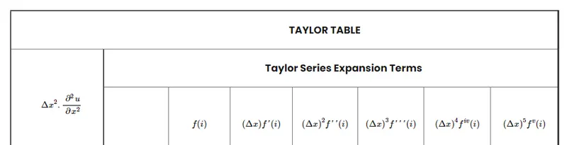
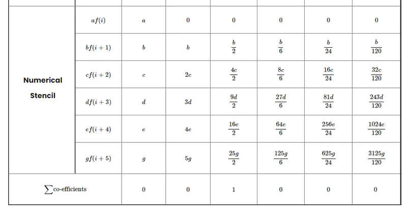
Equations:-

a+b+c+d+e+g = 0 ........(i)

0+b+2c+3d+4e+5g = 0 ........(ii)

0+b/2+4c/2+9d/2+16e/2+25g/2 = 1 ........(iii)

0+b/6+8c/6+27d/6+64e/6+125g/6 = 0 ........(iv)

0+b/24+16c/24+81d/24+256e/24+625g/24 = 0 ........(v)

0+b/120+32c/120+243d/120+1024e/120+3125g/120 = 0 ........(vi)

Writting the above equations in matrix form is slove for the a,b,c,d,e, and g

To get the all six equation solution in matrix form; AX=B

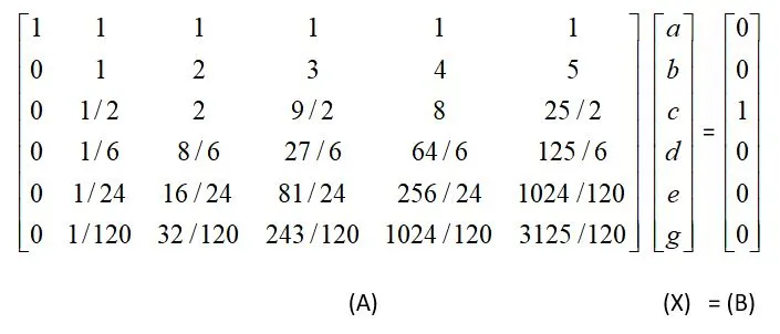
After solving the above the matrix we get value of all coefficients as;

a = 3.75000 or 15/4

b = -12.83333 or -77/6

c = 17.83333 or 107/6

d = -13.00000 or -13

e = 5.083333 or 61/21

g = -0.83333 or -5/6

there by substituting the above value in hyoithesis equation

taking L.C.M of the denominator trrms the fourth order approximation equation for second order derivative by Skewed right-sided difference method as follows

Skewed left-sided difference Method:-

It is refered to as Skewed left-sided difference method becouse it take the values from the current point as well as both the pravious points(L.H.S).

to derive 4th order Skewed left-sided difference method at point f(i) of function. since we are using Skewed left-sided difference method. here we have to define five points on the right of f(i). let those points be f(i-1), f(i-2), f(i-3), f(i-4), and f(i-5) with each a sapcing of (`(/_\\`x)`.

Number of node,

N = P+Q

where,

P = Order of derivative

Q = Order of approximation

as we are computing the 4th order approximation for 2nd order derivative we get,

N = 2+4

N = 6

therefore, this means that we required 6 nodes to get required accuracy.

there by formulating the hypothesis equation base on 6 nodes,

....(3)

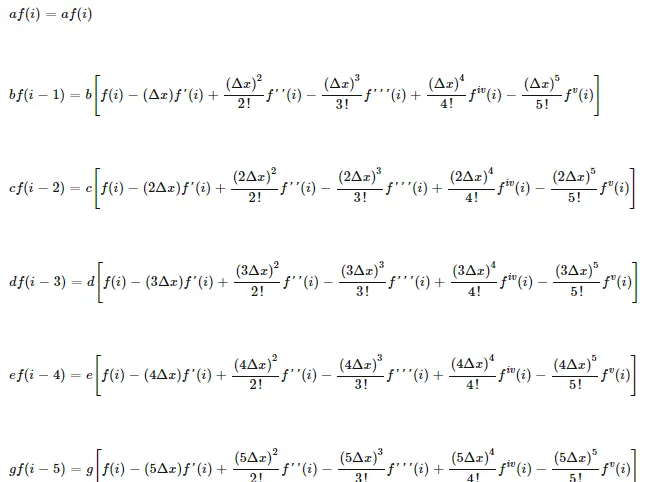
Taylor series expansion trems:-

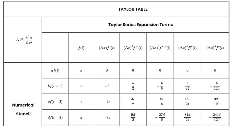
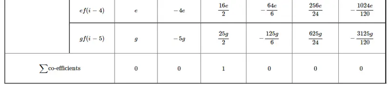
Taylor series tables:-

Equations:-

a+b+c+d+e+g = 0 ........(i)

0-b-2c-3d-4e-5g = 0 ........(ii)

0+b/2+4c/2+9d/2+16e/2+25g/2 = 1 ........(iii)

0-b/6-8c/6-27d/6-64e/6-125g/6 = 0 ........(iv)

0+b/24+16c/24+81d/24+256e/24+625g/24 = 0 ........(v)

0-b/120-32c/120-243d/120-1024e/120-3125g/120 = 0 ........(vi)

To get the all six equation solution in matrix form; AX=B

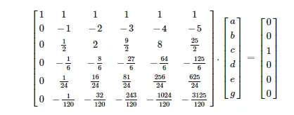
(A) (X) = (B)

After solving the above the matrix we get value of all coefficients as;

a = -3.75000 or -15/4

b = 12.83333 or 77/6

c = -17.83333 or -107/6

d = 13.00000 or 13

e =-5.083333 or -61/21

g = 0.83333 or 5/6

there by substituting the above value in hyoithesis equation

aking L.C.M of the denominator trrms the fourth order approximation equation for second order derivative by Skewed left-sided difference method as follows

Program and Explanation:-

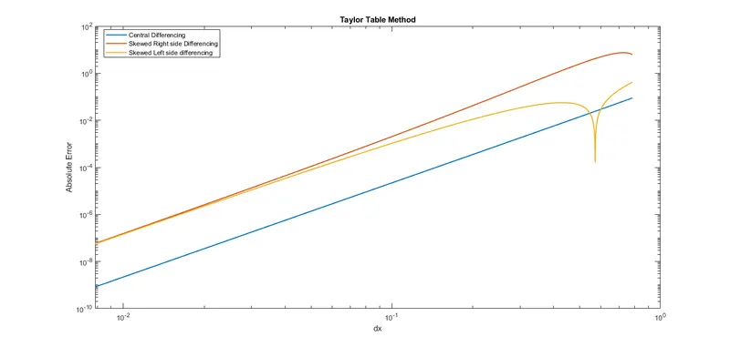
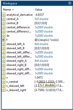
we are going to write a matlab program to compare the error of the function f(x) =e^x.cos(x), using the central difference, skewed right sided differencing and skewed left sided differencing method.

MATLAB Program:-

clear all

close all

clc

%inputs

x = pi/3;

dx = linspace(pi/4,pi/400,2000);

% analytical derivative

% using uv rule for f(x)

%Double differenting as we require seond order derivative

% f''(x) = -2*exp(x)*sin(x)

analytical_derivative = -2*exp(x)*sin(x);

% numerical derivative

% central defferencing method

% sloving for co-efficents from matrix form

% in from of Ax = B

central_A = [[1,1,1,1,1];[-2,-1,0,1,2];[2,1/2,0,1/2,2];[-8/6,-1/6,0,1/6,8/6];[16/24,1/24,0,1/24,16/24]];

central_B = [0;0;1;0;0];

x_central = inv(central_A)*central_B;

% skewed right sided differncing method

% solving for co-efficients from matrix form

% in form of Ax = B

skewed_right_A = [[1,1,1,1,1,1];[0,1,2,3,4,5];[0,1/2,2,9/2,8,25/2];[0,1/6,8/6,27/6,64/6,125/6];[0,1/24,16/24,81/24,256/24,625/24];[0,1/120,32/120,243/120,1024/120,3125/120]]

skewed_right_B = [0;0;1;0;0;0]

x_skewed_right = inv(skewed_right_A)*skewed_right_B

% skewed left sided differncing method

% solving for co-efficients from matrix form

% in form of Ax = B

skewed_left_A = [[1,1,1,1,1,1];[0,-1,-2,-3,-4,-5];[0,1/2,2,9/2,8,25/2];[0,-1/6,-8/6,-27/6,-64/6,-125/6];[0,1/24,16/24,81/24,256/24,625/24];[0,-1/120,-32/120,-243/120,-1024/120,-3125/120]]

skewed_left_B = [0;0;1;0;0;0]

x_skewed_left = inv(skewed_left_A)*skewed_left_B

% anonymous function

f = @(x) exp(x).*cos(x)

% difference approximation

central_difference = [(x_central(1)*f(x-(2.*dx))) + (x_central(2)*f(x-dx)) + (x_central(3)*f(x)) + (x_central(4)*f(x+dx)) + (x_central(5)*f(x+(2.*dx)))]./(dx.^2)

skewed_right_difference = ((x_skewed_right(1)*f(x)) + (x_skewed_right(2)*f(x+dx)) + (x_skewed_right(3)*f(x+(2.*dx))) + (x_skewed_right(4)*f(x+(3.*dx))) + (x_skewed_right(5)*f(x+(4.*dx))) + (x_skewed_right(6)*f(x+(5.*dx))))./(dx.^2)

skewed_left_difference = [(x_skewed_left(1)*f(x)) + (x_skewed_left(2)*f(x-dx)) + (x_skewed_left(3)*f(x-(2.*dx))) + (x_skewed_left(4)*f(x-(3.*dx))) + (x_skewed_left(5)*f(x-(4.*dx))) + ((x_skewed_left(6)*f(x-(5.*dx))))]./(dx.^2)

% computting absolute error

% error = numerical derivative - analytical derivative

central_differencing_error = abs(analytical_derivative - central_difference);

skewed_right_differencing_error = abs(analytical_derivative - skewed_right_difference)

skewed_left_differencing_error = abs(analytical_derivative - skewed_left_difference);

%plottibg error graph

loglog(dx,central_differencing_error,'LineWidth',1.5)

hold on

loglog(dx,skewed_right_differencing_error,'LineWidth',1.5)

hold on

loglog(dx,skewed_left_differencing_error,'LineWidth',1.5)

title('Taylor Table Method')

xlabel('dx')

ylabel('Absolute Error')

legend('Central Differencing','Skewed Right side Differencing','Skewed Left side differencing')

Explanation:-

the first step and most imporant step is clear all close all and clc commonds to clear . clear up window and workspace.

Input parameter x and dx in which linspace commond are use between pi/.4,pi/400, 2000, 2000 value are equally distributed values between pi/4 and pi/400.

obtain the analytical derivative of given function f(x) using uv rule for f(x) Double differenting as we require seond order derivative

f''(x) = -2*exp(x)*sin(x)

analytical_derivative = -2*exp(x)*sin(x)

we calculate unknown coefficents values of hypothesis euations for the central skewed right and skewed left differncing method numerical derivative

i sloving for co-efficents from matrix form

in from of Ax = B

after the obtaining all co efficients values all three defferncing method we define anonymous function handle f''. @operator ctreate the handle ans parentheses()after the operator .

anonymous function

f = @(x) exp(x).*cos(x)

next we calculated absulate error between the analytical derivative and obtain nrumical derivative.

finally ploting the log graph all three method central, skewed right side and skewed left side differencing method approximation error with respect to the range of dx

Plot:-

workspace:-

Why a skewed scheme is useful? What can a skewed scheme do that a CD scheme cannot?

The central method is more accurate and with minimum number of error compared to other difference methods of skewed scheme but central defferencing method need the values before and after it to compute. while if we need to compute at right end domain and we does not have any valued after the required derivative then we connot compute by central differencing we need to go skewed method only to get the result.

Conclusion:-

The taylors table for central right skewed and left skewed has been computed for 4th order with second order derivative and comparision for the same gas been done using plotting the graph.