Week 5.1 - Mid term project - Solving the steady and unsteady 2D heat conduction problem
Aim:
1. Steady-state analysis & Transient State Analysis
Solve the 2D heat conduction equation by using the point iterative techniques that were taught in the class. The Boundary conditions for the problem are as follows;
Top Boundary = 600 K
Bottom Boundary = 900 K
Left Boundary = 400 K
Right Boundary = 800 K
Introduction to Explicit Method:
Explicit methods
Explicit methods of body surfacing involve the use of mathematical approaches to define the body surface with parametric or polygonal patches. Polygons are commonly used to surface the body because they are the simplest geometric form (Volino & Magnenat-Thalmann, 2000). To define a surface using polygons, vertices making up the 3D body model (such as those defining cross-sections or 3D point clouds) are connected to form a mesh. These vertices may be moved independently to deform the mesh and provide new surface shape. The most common shapes are triangles or quadrangles, as these shapes easily lend themselves to geometrical computations used in mechanical modeling.
The explicit method allows solving problems element by element. Compared with the implicit method, it does not require the general matrix, since the velocity and displacement nodes can be counted directly, using the central difference integration scheme. However, the time step is limited by the size of the numerical stability. Accordingly, this method is considered as conditionally stable, because if the time step is too large, there will be a significant numerical error. In this method, there is no requirement for balance, so it is suitable for highly dynamic analysis, such as high velocity impact.
Implicit methods:
Implicit methods attempt to find a solution to the nonlinear system of equations iteratively by considering the current state of the system as well as its subsequent (or previous) time state. Newton-Raphson method or its modified forms are used to enforce equilibrium of the internal restoring forces with the externally applied loads. These incremental-iterative procedures are unconditionally stable which allows for using large increments. Hence, large incremental time steps can be applied in implicit schemes while maintaining numerical accuracy. However, the application of Newton-Raphson method or other iterative schemes within each time step increases the computational cost. While the approach works well for a broad range of problems, in severely nonlinear cases, it may fail to converge.
Matlab code:
clear all
close all
clc

%%inputs
nx = 20;
ny = nx;

tolerance = 1e-5;
error = 9e9;
T = 5;
dt = 1e-2;
x = linspace(0,1,nx);
y = linspace(0,1,ny);

%grid spacing
dx = x(2)-x(1);
dy = y(2)-y(1);

[xx,yy] = meshgrid(x,y);

%matrix difination
t = 300*ones(nx,ny);
t(end,:) = 900;
t(1,:) = 600;
t(:,end) = 800;
k = (2*(dx^2+dy^2)/(dx^2*dy^2));

t_old = t;
t_p = t;

method = 'which method ?'
solver = input(method);

%Jacobi

if solver ==1
    iter_1 = 1;
    tic;

    %convergence loop
    while (error>tolerance)
        for i = 2:(nx-1)
            for j = 2:(ny-1)
                TL = t_old(i-1,j);
                TR = t_old(i+1,j);
                TB = t_old(i,j-1);
                TT = t_old(i,j+1);

                H = (TL + TR )/dx^2;
                V = (TB + TT)/dy^2;

                t(i,j) = (H+ V)/k;
            end
        end
        time = toc;
        error = max(max(abs(t_old-t)));
        t_old = t;
        iter_1 = iter_1 + 1;
        [x,y] = contourf(xx,yy,t)
        colormap(jet)
        colorbar
        clabel(x,y)
        pause(0.03)
        title_text1 = sprintf('Steady state using jacobi = %d', iter_1);
        title_text2 = sprintf('Simulation time +%f s', time);
        title_text3 = sprintf('Final error = %f', error);
        title({title_text1; title_text2; title_text3})
    end
end

%Gauss siedel method
if solver ==2
    iter_2 = 1;
    tic;

    %convergence loop
    while (error>tolerance)
        for i = 2:(nx-1)
            for j = 2:(ny-1)
               %TL = t_old(i-1,j);
                TR = t_old(i+1,j);
                %TB = t_old(i,j-1);
                TT = t_old(i,j+1);

                H = (t(i-1,j)+ TR )/dx^2;
                V = (t(i,j-1) + TT)/dy^2;

                t(i,j) = (H+ V)/k;
            end
        end
        time2 = toc;
        error = max(max(abs(t_old-t)));
        t_old = t;
        iter_2 = iter_2 + 1;
        [x,y] = contourf(xx,yy,t)
        colormap(jet)
        colorbar
        clabel(x,y)
        pause(0.03)
        title_text1 = sprintf('Steady state using jacobi = %d', iter_2);
        title_text2 = sprintf('Simulation time +%f s', time2);
        title_text3 = sprintf('Final error = %f', error);
        title({title_text1; title_text2; title_text3})
    end
end

%%Successive over relaxaion (SOR) method
alpha = 0.3;
omega = 1.2;
if solver == 3
    iter_3 = 1;
    tic;
    %convergence loop
    while (error> tolerance)
          for i = 2:(nx-1)
            for j = 2:(ny-1)
               %TL = t_old(i-1,j);
                TR = t_old(i+1,j);
                %TB = t_old(i,j-1);
                TT = t_old(i,j+1);

                H = (t(i-1,j) + TR )/dx^2;
                V = (t(i,j-1) + TT)/dy^2;

                tgs(i,j) = (H+ V)/k;
                t(i,j) = (1-omega)*(t_old(i,j))+omega*tgs(i,j);
            end
        end
        time3 = toc;
        error = max(max(abs(t_old-t)));
        t_old = t;
        iter_3 = iter_3 + 1;
        [x,y] = contourf(xx,yy,t)
        colormap(jet)
        colorbar
        clabel(x,y)
        pause(0.03)
        title_text1 = sprintf('Steady state using jacobi = %d', iter_3);
        title_text2 = sprintf('Simulation time +%f s', time3);
        title_text3 = sprintf('Final error = %f', error);
        title({title_text1; title_text2; title_text3})
    end
end
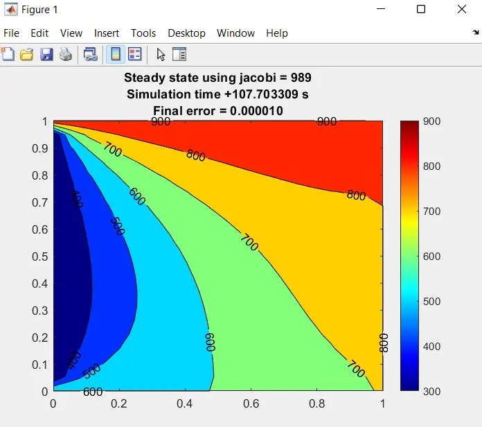
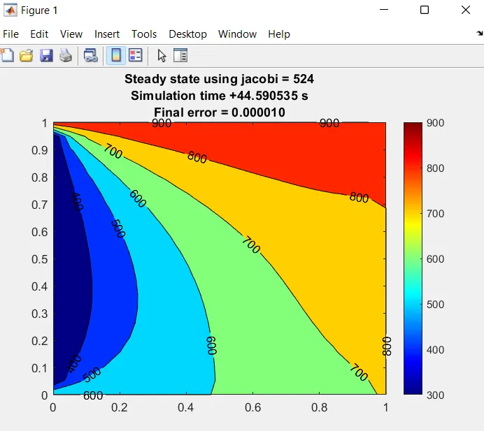
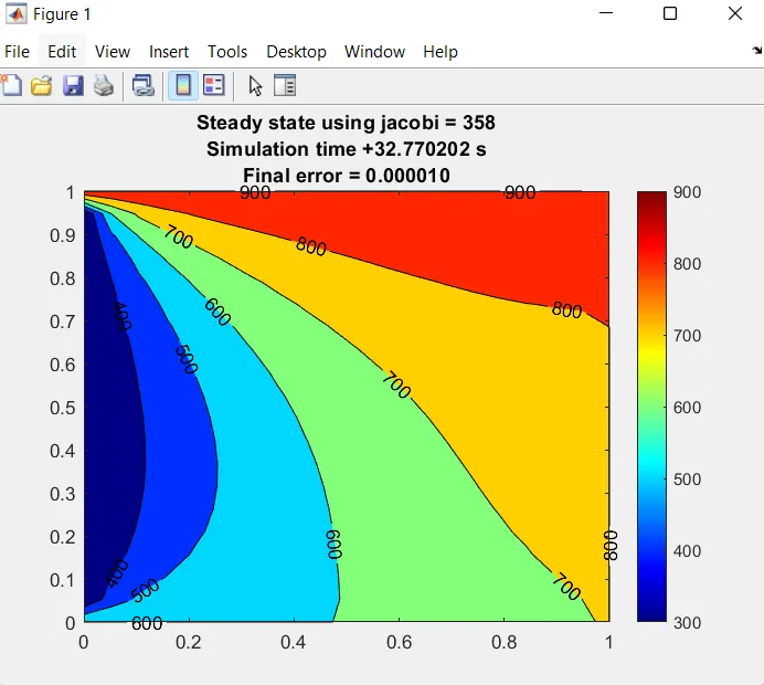
Output:
Matlab code:
clear all
close all
clc

%%inputs
nx = 20;
ny = nx;
alpha = 1.4;
omega = 1.2;

tolerance = 1e-5;
error = 9e9;
T = 5;
dt = 1e-2;
x = linspace(0,1,nx);
y = linspace(0,1,ny);

%grid spacing
dx = x(2)-x(1);
dy = y(2)-y(1);

[xx,yy] = meshgrid(x,y);

%matrix difination
t = 300*ones(nx,ny);
t(end,:) = 900;
t(1,:) = 600;
t(:,end) = 800;
k1 = alpha*dt/dx^2;
k2 = alpha*dt/dy^2;
k = 1+(2*k1)+(2*k2);

t_old = t;
t_p = t;

method = 'which method ?'
solver = input(method);

%Jacobi

if solver ==1
    iter_1 = 1;
    tic;

    %convergence loop
    while (error>tolerance)
        for i = 2:(nx-1)
            for j = 2:(ny-1)
                TL = t_old(i-1,j);
                TR = t_old(i+1,j);
                TB = t_old(i,j-1);
                TT = t_old(i,j+1);

                H = TL + TR;
                V = TB + TT;

                t(i,j) = ((t_p(i,j)+H*k1 +V*k2)/k);
            end
        end
        time = toc;
        error = max(max(abs(t_old-t)));
        t_old = t;
        iter_1 = iter_1 + 1;
        [x,y] = contourf(xx,yy,t)
        colormap(jet)
        colorbar
        clabel(x,y)
        pause(0.03)
        title_text1 = sprintf('Steady state using jacobi = %d', iter_1);
        title_text2 = sprintf('Simulation time +%f s', time);
        title_text3 = sprintf('Final error = %f', error);
        title({title_text1; title_text2; title_text3})
    end
end

%Guass siedel method
if solver ==2
    iter_2 = 1;
    tic;

    %convergence loop
    while (error>tolerance)
        for i = 2:(nx-1)
            for j = 2:(ny-1)
                TL = t_old(i-1,j);
                TR = t_old(i+1,j);
                TB = t_old(i,j-1);
                TT = t_old(i,j+1);

                H = t(i-1,j) + TR;
                V = t(i,j-1) + TT;

                t(i,j) = ((t_p(i,j)+H*k1 +V*k2)/k);
            end
        end
        time2 = toc;
        error = max(max(abs(t_old-t)));
        t_old = t;
        iter_2 = iter_2 + 1;
        [x,y] = contourf(xx,yy,t)
        colormap(jet)
        colorbar
        clabel(x,y)
        pause(0.03)
        title_text1 = sprintf('Steady state using jacobi = %d', iter_2);
        title_text2 = sprintf('Simulation time +%f s', time2);
        title_text3 = sprintf('Final error = %f', error);
        title({title_text1; title_text2; title_text3})
    end
end

%%Successive over relaxation (SOR) method
if solver ==3
    iter_3 = 1;
    tic;

    %convergence loop
    while (error>tolerance)
        for i = 2:(nx-1)
            for j = 2:(ny-1)
                TL = t_old(i-1,j);
                TR = t_old(i+1,j);
                TB = t_old(i,j-1);
                TT = t_old(i,j+1);

                H = t(i-1,j) + TR;
                V = t(i,j-1) + TT;

                tgs(i,j) = ((t_p(i,j)+H*k1 +V*k2)/k);
                t(i,j) = (1-omega)*(t_old(i,j)) + omega*tgs(i,j);
            end
        end
        time3 = toc;
        error = max(max(abs(t_old-t)));
        t_old = t;
        iter_3 = iter_3 + 1;
        [x,y] = contourf(xx,yy,t)
        colormap(jet)
        colorbar
        clabel(x,y)
        pause(0.03)
        title_text1 = sprintf('Steady state using jacobi = %d', iter_3);
        title_text2 = sprintf('Simulation time +%f s', time3);
        title_text3 = sprintf('Final error = %f', error);
        title({title_text1; title_text2; title_text3})
    end
end
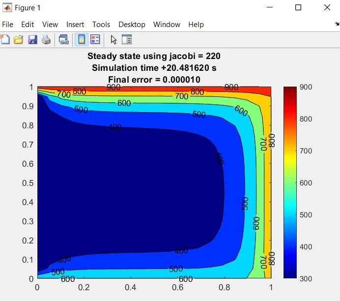
Plots:
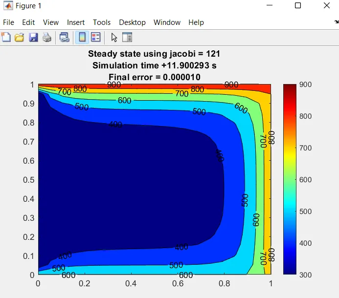
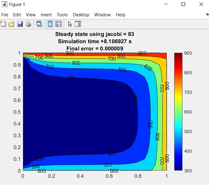
Matlab code:
clear all
close all
clc

%%inputs
nx = 10;
ny = nx;
alpha = 0.3;
omega = 1.2;

tolerance = 1e-5;
error = 9e9;
T = 5;
dt = 0.01;
nt = T/dt;
x = linspace(0,1,nx);
y = linspace(0,1,ny);

%grid spacing
dx = x(2)-x(1);
dy = y(2)-y(1);

[xx,yy] = meshgrid(x,y);

%matrix difination
t = 300*ones(nx,ny);
t(end,:) = 900;
t(1,:) = 600;
t(:,end) = 800;
k1 = alpha*dt/dx^2;
k2 = alpha*dt/dy^2;
k = 1+(2*k1)+(2*k2);

t_old = t;
t_p = t;

method = 'which method ?'
solver = input(method);

%Jacobi

if solver ==1
    iter_1 = 1;
    nt = T/dt;
    tic;
    for m = 1:nt
    %convergence loop
    while (error>tolerance)
        for i = 2:(nx-1)
            for j = 2:(ny-1)
                TL = t_old(i-1,j);
                TR = t_old(i+1,j);
                TB = t_old(i,j-1);
                TT = t_old(i,j+1);

                H = TL + TR;
                V = TB + TT;

                t(i,j) = ((t_p(i,j)+H*k1 +V*k2)/k);
            end
        end
         error = max(max(abs(t_old-t)));
        t_old = t;
        iter_1 = iter_1 + 1;
    end
    t_p = t;
    end
        time = toc;
        [x,y] = contourf(xx,yy,t)
        colormap(jet)
        colorbar
        clabel(x,y)
        pause(0.03)
        title_text1 = sprintf('Steady state using jacobi = %d', iter_1);
        title_text2 = sprintf('Simulation time +%f s', time);
        title_text3 = sprintf('Final error = %f', error);
        title({title_text1; title_text2; title_text3})
    end


%Guass siedel method
if solver ==2
    iter_2 = 1;
    tic;

    for m = 1:nt
    %convergence loop
    while (error>tolerance)
        for i = 2:(nx-1)
            for j = 2:(ny-1)
                TL = t_old(i-1,j);
                TR = t_old(i+1,j);
                TB = t_old(i,j-1);
                TT = t_old(i,j+1);

                H = t(i-1,j) + TR;
                V = t(i,j-1) + TT;

                t(i,j) = ((t_p(i,j)+H*k1 +V*k2)/k);
            end
        end
         error = max(max(abs(t_old-t)));
        t_old = t;
        iter_2 = iter_2 + 1;
    end
    t_p = t;
    end
        time2 = toc;
        [x,y] = contourf(xx,yy,t)
        colormap(jet)
        colorbar
        clabel(x,y)
        pause(0.03)
        title_text1 = sprintf('Steady state using jacobi = %d', iter_2);
        title_text2 = sprintf('Simulation time +%f s', time2);
        title_text3 = sprintf('Final error = %f', error);
        title({title_text1; title_text2; title_text3})
end

%%Successive over relaxation (SOR) method
if solver ==3
    iter_3 = 1;
    tic;
    for m = 1:nt
    %convergence loop
    while (error>tolerance)
        for i = 2:(nx-1)
            for j = 2:(ny-1)
                TL = t_old(i-1,j);
                TR = t_old(i+1,j);
                TB = t_old(i,j-1);
                TT = t_old(i,j+1);

                H = t(i-1,j) + TR;
                V = t(i,j-1) + TT;

                tgs(i,j) = ((t_p(i,j)+H*k1 +V*k2)/k);
                t(i,j) = (1-omega)*(t_old(i,j)) + omega*tgs(i,j);
            end
        end
         error = max(max(abs(t_old-t)));
        t_old = t;
        iter_3 = iter_3 + 1;
    end
    t_p = t;
    end
        time3 = toc;

        [x,y] = contourf(xx,yy,t)
        colormap(jet)
        colorbar
        clabel(x,y)
        pause(0.03)
        title_text1 = sprintf('Steady state using jacobi = %d', iter_3);
        title_text2 = sprintf('Simulation time +%f s', time3);
        title_text3 = sprintf('Final error = %f', error);
        title({title_text1; title_text2; title_text3})
    end
Plots:
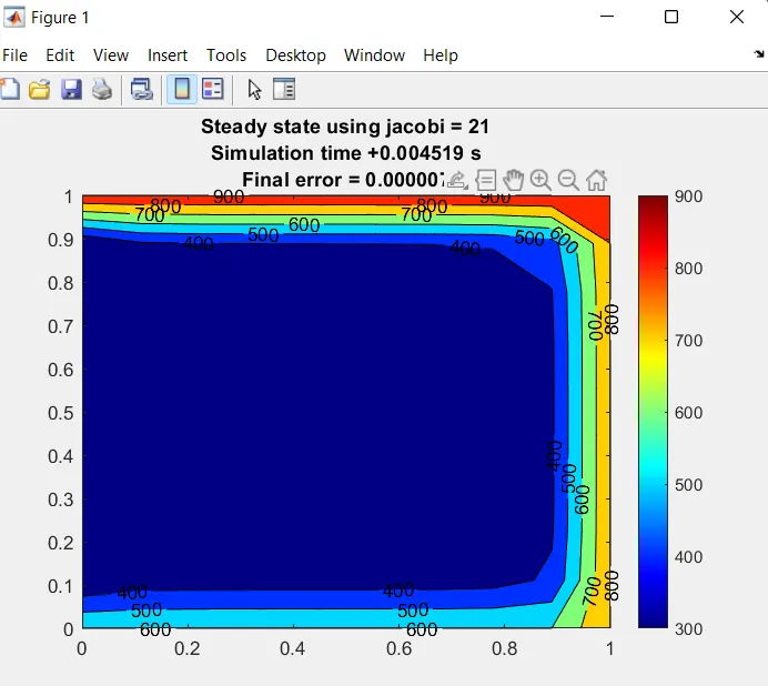
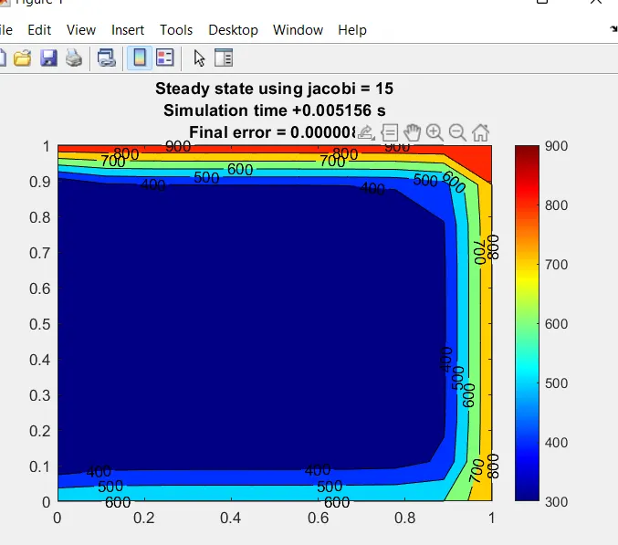
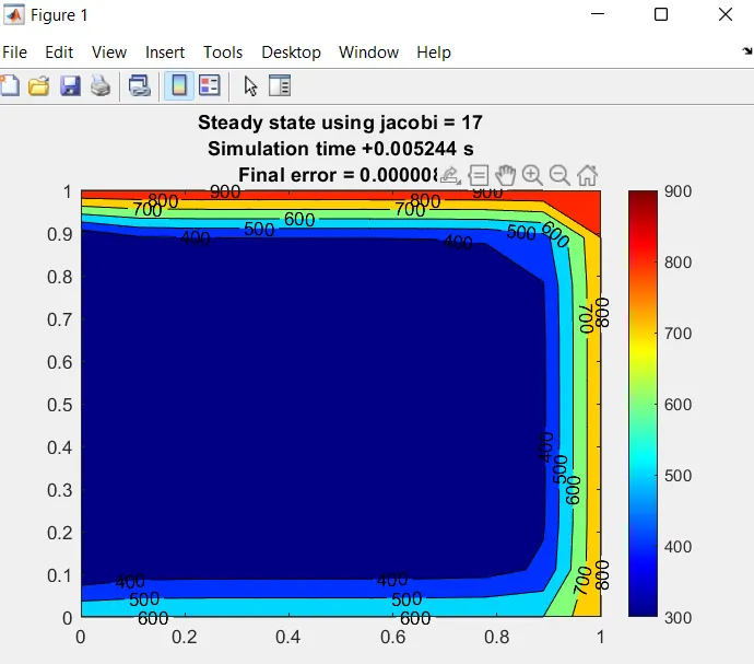
Conclusion:
Comparing the different iterations approaches and states, we can conclude the following things
The computational time and iteration required are SOR<GS<JACOBI for both steady and unsteady states.
Steady states are less complicated to analyze because time marching properties change has been avoided, on the other hand, the Transient approach deals with more sophisticated and complicated unknowns and considerations of time marching phenomenon change such as diffusion rates.
Between Explicit and implicit results, the latter does not depend greatly on the Courant number for its stability and convergence, on the other hand in the Explicit approach information from a given cell or mesh element must propagate ot its immediate neighbors, hence the low CFL number needs to be considered.