Week 5.1 - Mid term project - Solving the steady and unsteady 2D heat conduction problem
AIM: Solve the 2D heat conduction equation by using Jacobi, Gauss-seidel and Successive over relaxation methods.
GOVERNING EQUATIONS:
Conduction is process of heat transfer in solids and the general equation for same is,
`(delT)/(delt) - alpha((del^2T)/(delx^2) + (del^2T)/(dely^2) + (del^2T)/(delz^2)) = 0`
As for the project the we have taken 2D heat conduction hence equation becomes
`(delT)/(delt) - alpha((del^2T)/(delx^2) + (del^2T)/(dely^2)) = 0`
This form of equation is in transient form.
Implicit form of same is, `Tp^(n+1) = (1/[1+2k1+2k2])(Tp^n + k1(Tl^(n+1) + Tr^(n+1)) + k2(Tt^(n+1) + Tb^(n+1)))`
In explicit form it will be, `Tp^(n+1) = (1/[1+2k1+2k2])(Tp^n + k1(Tl^(n) + Tr^(n)) + k2(Tt^(n) + Tb^(n)))`
The steady state form of the equation is,
`(del^2T)/(delx^2) + (del^2T)/(dely^2) = 0`
MATLAB CODE :
FOR STEADY STATE
clear all
close all
clc

% Number of nodes(discretization length) and Domain length
no_of_node = 10;
domain_length = 1;
%coordinate values of nodes in the discretized domain
x = linspace(0,domain_length,no_of_node);
y = linspace(0,domain_length,no_of_node);
dx = domain_length/(no_of_node - 1);
dy = domain_length/(no_of_node - 1);

%Guess temperature value at all nodes
T = 300*ones(no_of_node,no_of_node);
%Boundary conditions
T(1:end,1) = 400; %left
T(1:end,end) = 800; %right
T(1,1:end) = 900; %bottom
T(end,1:end) = 600; %top
%Boundary condition od corner nodes
T(1,1) = 500;
T(end,1) = 650;
T(1,end) = 700;
T(end,end) = 850;
%assigning t_old
T_old = T;
%constant values
K = (2*(dx^2 + dy^2))/(dx^2*dy^2);
O = 1.2; %omega value
%Initialising error and tolerance values for looping conditions
error = 100;
tol = 1e-4;
no_of_iter = 0;

%Starting convergence loop
Iteration_technique = input('(1) for Jacobi, (2) for GS, (3) for SOR');
%Jacobi method
if Iteration_technique == 1
    while (error>tol)
        for i = 2:no_of_node-1
            for j = 2:no_of_node-1
                T(i,j) = ((T_old(i+1,j)+T_old(i-1,j))/dx^2+(T_old(i,j+1)+T_old(i,j-1))/dy^2)/K;
            end
        end
        error = max(max(abs(T_old-T)));
        %updating T_old
        T_old = T;
        no_of_iter = no_of_iter + 1;
    end
%GS Method
elseif Iteration_technique == 2
        while (error>tol)
        for i = 2:(no_of_node-1)
            for j = 2:(no_of_node-1)
                T(i,j) = (((T_old(i+1,j)+T(i-1,j))/dx^2) + ((T_old(i,j+1)+T(i,j-1))/dy^2))/K;
            end
        end
        error = max(max(abs(T_old-T)));
        %updating T_old
        T_old = T;
        no_of_iter = no_of_iter + 1;
        end


    else
         while (error>tol)
        for i = 2:(no_of_node-1)
            for j = 2:(no_of_node-1)
                T(i,j) = ((1-O)*T_old(i,j))+(O*(((T_old(i+1,j)+T(i-1,j))/dx^2) + ((T_old(i,j+1)+T(i,j-1))/dy^2))/K);
            end
        end
        error = max(max(abs(T_old-T)));
        %updating T_old
        T_old = T;
        no_of_iter = no_of_iter + 1;
         end
end

    [X,Y] = meshgrid(x,y);
    contourf(X,Y,T)
    colorbar
CODE EXPLANATION
Input values are defined for the respected variables and Temperature matrix is created.
After that we include the boundary conditions as well as average temperature values for all the corner nodes into the temperature matrix.
Constant values of Omega(O), tolerance(tol) are defined to initialise the convergence loop.
User provides the input on which iterative method will be used for convergence
In the loop, if else statement is used to solve the heat conduction steady state equations by the selected method of iteration.
While loop is used to keep the convergence loop iterating till we achieve the or converge to required tolerance value.
As the problem is of two dimensions two for loop are used to calculate temperature values at every node in each itterative method.
Meshgrid of x and y is created to form the domain or the 2D plane where distribution of temperature is plotted using contourf command.
FOR TRANSIENT FORM
clear all
close all
clc

% Number of nodes(discretization length) and Domain length
no_of_node = 10;
domain_length = 1;
%coordinate values of nodes in the discretized domain
x = linspace(0,domain_length,no_of_node);
y = linspace(0,domain_length,no_of_node);
dx = domain_length/(no_of_node - 1);
dy = domain_length/(no_of_node - 1);
dt = 0.1;

%Guess temperature value at all nodes
T = 300*ones(no_of_node,no_of_node);
%Boundary conditions
T(1:end,1) = 400; %left
T(1:end,end) = 800; %right
T(1,1:end) = 900; %bottom
T(end,1:end) = 600; %top
%Boundary condition od corner nodes
T(1,1) = 500;
T(end,1) = 650;
T(1,end) = 700;
T(end,end) = 850;

%assigning t_old
T_old = T;
%assigning T for previous time step
T_prev = T;

%constant values
O = 1.2; %omega value
A = 1.5; %Alpha value
K1 = (A*dt)/(dx^2);
K2 = (A*dt)/(dy^2);

%Initialising error and tolerance values for looping conditions
error = 100;
tol = 1e-4;
no_of_iter = 0;

%Starting convergence loop
Approach = input('1 for implicit or 2 for explicit')
if Approach == 1
    iteration_technique = input('1 for Jacobi 2 for GS 3 for SOR')
    if iteration_technique == 1
        for nt = 1:1500 %JACOBI
            while(error>tol)
                for i = 2:no_of_node-1
                    for j = 2:no_of_node-1
                        term1 = 1/(1+(2*K1)+(2*K2));
                        term2 = K1*(T_old(i+1,j)+T_old(i-1,j));
                        term3 = K2*(T_old(i,j+1)+T_old(i,j-1));
                        T(i,j) = term1*(T_prev(i,j)+term2+term3);
                    end
                end
                no_of_iter= no_of_iter+1;
                error = max(max((abs(T_old-T))));
                T_old = T;
            end
            T_prev = T;
        end
    elseif iteration_technique == 2
        for nt = 1:1500 %GS
             while(error>tol)
                for i = 2:no_of_node-1
                    for j = 2:no_of_node-1
                        term1 = 1/(1+(2*K1)+(2*K2));
                        term2 = K1*(T_old(i+1,j)+T(i-1,j));
                        term3 = K2*(T_old(i,j+1)+T(i,j-1));
                        T(i,j) = term1*(T_prev(i,j)+term2+term3);
                    end
                end
                no_of_iter= no_of_iter+1;
                error = max(max((abs(T_old-T))));
                T_old = T;
             end
            T_prev = T;
        end
    else
        for nt = 1:1500 %SOR
            while(error>tol)
                 for i = 2:no_of_node-1
                    for j = 2:no_of_node-1
                        term1 = 1/(1+(2*K1)+(2*K2));
                        term2 = K1*(T_old(i+1,j)+T(i-1,j));
                        term3 = K2*(T_old(i,j+1)+T(i,j-1));
                        term4 = term1*(T_prev(i,j)+term2+term3);
                        T(i,j) = (1-O)*T_old(i,j)+(O*term4);
                    end
                end
                no_of_iter= no_of_iter+1;
                error = max(max((abs(T_old-T))));
                T_old = T;
            end
             T_prev = T;
        end
    end
else
    for nt = 1:1500 %EXPLICIT
         for i = 2:no_of_node-1
                    for j = 2:no_of_node-1
                        term1 = K1*(T_prev(i+1,j)-2*T_prev(i,j)+T_prev(i-1,j));
                        term2 = K2*(T_prev(i,j+1)-2*T_prev(i,j)+T_prev(i,j-1));
                        T(i,j) = T_prev(i,j)+term1+term2;
                    end
         end

          T_prev = T;
         no_of_iter = no_of_iter + 1;
    end

end
%plotting outcome
[X,Y] = meshgrid(x,y);
contourf(X,Y,T)
colorbar
CODE EXPLANATION
Input values are defined for the respected variables and Temperature matrix is created.
After that we include the boundary conditions as well as average temperature values for all the corner nodes into the temperature matrix.
Constant values of Omega(O), tolerance(tol) and Alpha(A) are defined to initialise the convergence loop.
The user inputs the approach and technique to be used.
In the loop, if else statement is used to solve the heat conduction steady state equations by the selected method of iteration as well as approach for the probelm.
While loop is used to keep the convergence loop iterating till we achieve the or converge to required tolerance value.
As the problem is of two dimensions two for loop are used to calculate temperature values at every node in each itterative method.
Meshgrid of x and y is created to form the domain or the 2D plane where distribution of temperature is plotted using contourf command.
OUTPUT PLOT:
STEADY STATE
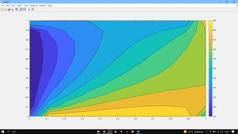
NUMBER OF ITERATION FOR JACOBI = 207
NUMBER OF ITERATION FOR GAUSS-SIEDEL = 111
NUMBER OF ITERATION FOR SOR = 74
TRANSIENT FORM
IN IMPLICIT,
NUMBER OF ITERATION FOR JACOBI = 156
NUMBER OF ITERATION FOR GAUSS-SIEDEL = 84
NUMBER OF ITERATION FOR SOR = 56
IN EXPLICIT
NUMBER OF ITERATIONS = 1500(due to number of time steps)
CONCLUSION
Both the programs were successfuly executed and output plots were obtained.
As from the attached images we can observe that output for both Steady and transient state are same as in the transient form implicit approach the solution approaches the steady state.
The edges of contour plot display the boundary conditions.
Also we observed for all cases number of iterations of SOR<GS<JACOBI.