Week 5.1 - Mid term project - Solving the steady and unsteady 2D heat conduction problem
PROJECT-
- To solve the 2D heat conduction equation by using jacobi , Gauss-Seidel & Succesive over relaxation for implicit and explicit schemes using Matlab .
THEORY-
-There are two condition for 2D heat conduction.
- Steady state condition
- Unsteady / Transient conditon
- In steady state the heat transfer process that does not get affected by the time interval is known as steady-state heat transfer. In this type of heat transfer, the temperature of the object does not change with respect to time.
-Unsteady state condition are a presurcor to steady state condition,the heat transfer process that gets affected by the time interval is known as the unsteady state . In this type of heat transfer, the temperature of the object increases or decreases with respect to time.
-For 2D heat conduction equation we are using some method as follow as,
- Jacobi- The Jacobi method is an algorithm in linear algebra for determining the solutions of a system of linear equations with largest absolute values in each row and column dominated by the diagonal element. Each diagonal element is solved for, and an approximate value given. The process is then iterated until it converge.
- Gauss-seidel- The method is similar to the jacobi and in the same way strict or irreducible diagonal dominance of the system is sufficient to ensure but after each iteration the temperature value is updated to the previous iteration.
- Succesive over relaxation-Generaly this metod is used to enhance the method od jacobi and guss seidel method. when the relaxation factor is less than 1 the iteration is under relax, if the relaxatio factor is greater the 1 the iteration is over relax. so the value of relaxtion factor taken to be 1.1 or 1.2
OBJECTIVE-
-Boundary conditions for the problem,
- Left boundary(T_L) = 400k
- Top boundary(T_T) = 600k
- Right boundary(T_R) = 800k
- Bottom boundary(T_B) = 9
-From the boundary condition we can calculate the central temprature ,
`Tp = 1/k*[(TL +TR)/(Deltax^2)+(T T+TB)/(Deltay^2)]`
-Computaion area should be a square.
- Number of points on x direction is equal to the number of point in y direction , so we assume nx=ny.
- nx=ny = 10
- The 2D transient equation
`(DT)/(Dt) + alpha((del^2T)/(delx^2 ) +(del^2T)/(dely^2)) = 0`
- The steady state equation
`(del^2T)/(delx^2) +(delT)/(dely^2) = 0`
PROGRAM FOR STEADY STATE EQUATION-
JACOBI ITERATIION
clear all
close all
clc
%Solving the steady state 2D heat conduction
%jacobi method

%inputs
L=1;
%Number of nodes along x and y diretion
nx=10;
ny=nx;

%change of x w.r.t x coordinate
dx=L/(nx-1);
%change of x w.r.t x coordinate
dy=L/(ny-1);

x=linspace(0,1,nx)
y=linspace(0,1,ny);

%defining boundary condition
T_L = 400;
T_T = 600;
T_R = 800;
T_B = 900;
%Temperature array
T = 300*ones(nx,ny);

%Updating the value of temperature
T(2:ny - 1,1) = T_L;
T(2:ny - 1,nx) = T_R;
T(1,2:nx-1) = T_T;
T(ny,2:nx-1) = T_B;

% Calculating the avg temperature at cornors
T(1,1) = (T_T + T_L)/2;
T(nx,ny) = (T_R + T_B)/2;
T(1,ny) = (T_T + T_R)/2;
T(nx,1) = (T_L + T_B)/2;

%Assigning the original value to T
T_intial = T;
T_old = T;

iterative_solver = 1;
error = 9e9;
tol = 1e-4;

%jacobi method
tic;
if iterative_solver == 1;
    jacobi_itration = 1;

    while(error>tol)

        for i = 2:nx - 1
            for j = 2:ny - 1
            T(i,j) = 0.25*(T_old(i-1,j)+T_old(i+1,j)+T_old(i,j-1)+T_old(i,j+1))
            end
        end
        error = max(max(abs(T_old-T)));
        T_old = T;
        jacobi_itration = jacobi_itration + 1;

    end
end
F = toc;
%ploting the figure
figure(1)
contourf(x,y,T)
clabel(contourf(x,y,T))
colorbar
colormap("jet")
set(gca,'ydir', 'reverse')
xlabel('X')
ylabel('Y')
title(sprintf('Number of jacobi itration(implicit)=%d,computation time = %f',jacobi_itration,F));
pause(0.03)
RESULT-
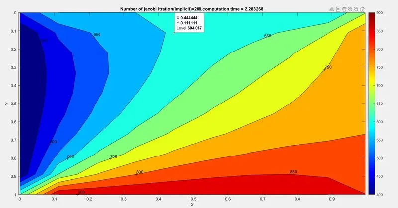
GAUSS-SEIDEL ITERATION
clear all
close all
clc
%Solving the steady state 2D heat conduction
%gs method

%inputs
L=1;
%Number of nodes along x and y diretion
nx=10;
ny=nx;

%change of x w.r.t x coordinate
dx=L/(nx-1);
%change of x w.r.t x coordinate
dy=L/(ny-1);

x=linspace(0,1,nx)
y=linspace(0,1,ny);

%defining boundary condition
T_L = 400;
T_T = 600;
T_R = 800;
T_B = 900;
%Temperature array
T = 300*ones(nx,ny);

%Updating the value of temperature
T(2:ny - 1,1) = T_L;
T(2:ny - 1,nx) = T_R;
T(1,2:nx-1) = T_T;
T(ny,2:nx-1) = T_B;

% Calculating the avg temperature at cornors
T(1,1) = (T_T + T_L)/2;
T(nx,ny) = (T_R + T_B)/2;
T(1,ny) = (T_T + T_R)/2;
T(nx,1) = (T_L + T_B)/2;

%Assigning the original value to T
T_intial = T;
T_old = T;

iterative_solver = 2;
error = 9e9;
tol = 1e-4;

%Gauss-seidel method
tic;
if iterative_solver == 2;
    gs_iteration = 1;

    while(error>tol)

        for i = 2:nx - 1
            for j = 2:ny - 1
            T(i,j) = 0.25*(T(i-1,j)+T_old(i+1,j)+T(i,j-1)+T_old(i,j+1))
            end
        end
        error = max(max(abs(T_old-T)));
        T_old = T;
        gs_iteration = gs_iteration + 1;

    end
end
F = toc;
%ploting the figure
figure(2)
contourf(x,y,T)
clabel(contourf(x,y,T))
colorbar
colormap("jet")
set(gca,'ydir', 'reverse')
xlabel('X')
ylabel('Y')
title(sprintf('Number of gs itration(implicit)=%d,computation time = %f',gs_iteration,F));
pause(0.03)
RESULT-
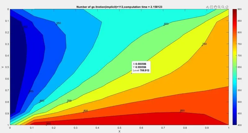
SUCCESIVE OVER RELAXATION-
clear all
close all
clc
%Solving the steady state 2D heat conduction
%Succesive over relaxation method

%inputs
L=1;
%Number of nodes along x and y diretion
nx=10;
ny=nx;


%change of x w.r.t x coordinate
dx=L/(nx-1);
%change of x w.r.t x coordinate
dy=L/(ny-1);

x=linspace(0,1,nx)
y=linspace(0,1,ny);

%defining boundary condition
T_L = 400;
T_T = 600;
T_R = 800;
T_B = 900;
%Temperature array
T = 300*ones(nx,ny);

%Updating the value of temperature
T(2:ny - 1,1) = T_L;
T(2:ny - 1,nx) = T_R;
T(1,2:nx-1) = T_T;
T(ny,2:nx-1) = T_B;

% Calculating the avg temperature at cornors
T(1,1) = (T_T + T_L)/2;
T(nx,ny) = (T_R + T_B)/2;
T(1,ny) = (T_T + T_R)/2;
T(nx,1) = (T_L + T_B)/2;

iterative_solver = 3;
error = 9e9;
tol = 1e-4;
omega = 1.1

%Assigning the original value to T
T_intial = T;
T_old = T;

%sor method
tic;
if iterative_solver == 3;
    sor_itration = 1;

    while(error>tol)

        for i = 2:nx - 1
            for j = 2:ny - 1
            T(i,j) = (1-omega)*T_old(i,j)+omega*(0.25*(T(i-1,j)+T_old(i+1,j)+T(i,j-1)+T_old(i,j+1)));
            end
        end
        error = max(max(abs(T_old-T)));
        T_old = T;
        sor_itration = sor_itration + 1;

    end
end
F = toc;
%ploting the figure
figure(1)
contourf(x,y,T)
clabel(contourf(x,y,T))
colorbar
colormap("jet")
set(gca,'ydir', 'reverse')
xlabel('X')
ylabel('Y')
title(sprintf('Number of sor itration(implicit)=%d,computation time = %f',sor_itration,F));
pause(0.03)
RESULT-
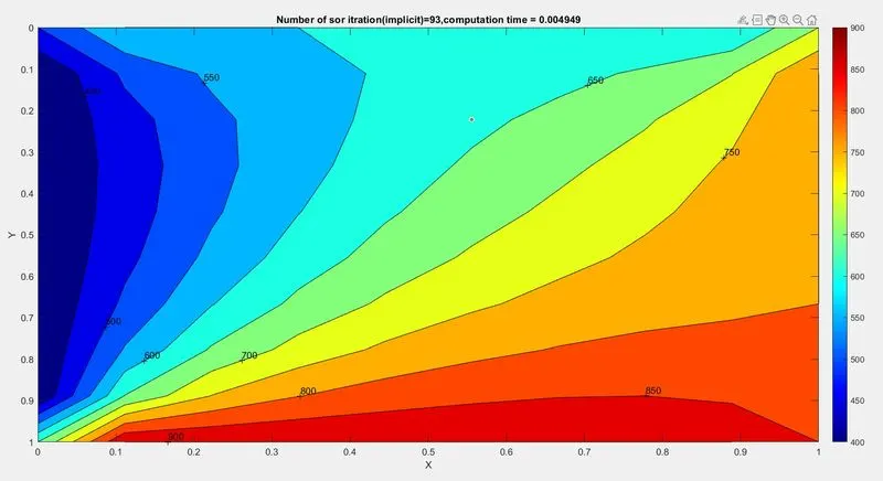
STEADY STATE RESULT-
TYPES OF SCHEMES ITERATION NUMBER COMPUTION TIME
JACOBI 208 2.28
GAUSS-SEDEL 112 2.15
SUCCESIVE OVER RELAXATION 93 0.0049
UNSTEADY /TRANSIENT STATE CONDITION
Unsteady state condition are a presurcor to steady state condition,the heat transfer process that gets affected by the time interval is known as the unsteady state . In this type of heat transfer, the temperature of the object increases or decreases with respect to time
- 2D tranisient equation
`(delT)/(delt) + alpha((del^2T)/(delx^2 ) +(del^2T)/(dely^2)) = 0`
-Descritize the equation it becomes,
`Tundersetpoverset(n+1)`=`Tundersetp oversetn`+`k1*(TundersetL`-`2*TundersetP`+`TundersetR``(n) +k2(TundersetT`-`2*TundersetP`+`TundrsetB)``(n)`
where k1 and k2 are CFL value of x and y direction
`K1 = alpha*(Deltat)/(Deltax^2)`
`K2 = alpha*(Deltat)/(Deltay^2`
JACOBI ITERATION
clear all
close all
clc
%Solving the steady state 2D heat conduction
%jacobi method(explicit)
%inputs
L=1;
%Number of nodes along x and y diretion
nx=10;
ny=nx;
nt=1400
alpha = 1.2
%change of x w.r.t x coordinate
dx=L/(nx-1);
%change of x w.r.t x coordinate
dy=L/(ny-1);
x=linspace(0,1,nx)
y=linspace(0,1,ny);
%defining boundary condition
T_L = 400;
T_T = 600;
T_R = 800;
T_B = 900;
%Temperature array
T = 300*ones(nx,ny);
%Updating the value of temperature
T(2:ny - 1,1) = T_L;
T(2:ny - 1,nx) = T_R;
T(1,2:nx-1) = T_T;
T(ny,2:nx-1) = T_B;
% Calculating the avg temperature at cornors
T(1,1) = (T_T + T_L)/2;
T(nx,ny) = (T_R + T_B)/2;
T(1,ny) = (T_T + T_R)/2;
T(nx,1) = (T_L + T_B)/2;
iterative_solver = 3;
error = 9e9;
tol = 1e-4;
dt = 1e-3
%Assigning the original value to T
T_intial = T;
T_old = T;
% CFL numbers
k1 = (alpha*dt)/dx^2;
k2 = (alpha*dt)/dy^2;
%jacobi method(explicit)
tic;
jacobi_iteration = 1;
for k = 1:nt
error = 9e9;
while(error>tol)
for i = 2:nx-1
for j = 2:ny-1
term1 = 1/(1+(2*k1)+(2*k2));
term2 = k1*term1
term3 = k2*term1
H = (T_old(i-1,j)) + (T_old(i+1,j))
V = (T_old(i,j+1)) + (T_old(i,j-1))
T(i,j) = (T_intial(i,j)*term1) +(H*term2) + (V*term3)
end
end
error = max(max(abs(T_old-T)));
T_old = T;
jacobi_iteration = jacobi_iteration+1
end
T_intial = T;
F = toc;
%ploting the figure
figure(1)
contourf(x,y,T)
clabel(contourf(x,y,T))
colorbar
colormap("jet")
set(gca,'ydir', 'reverse')
xlabel('X')
ylabel('Y')
title(sprintf('Number of jacobi itration(implicit)=%d,computation time = %f',jacobi_iteration,F));
pause(0.03)
end
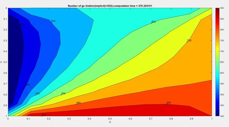
RESULT-
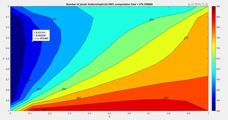
GAUSS-SEIDEL ITERATION
clear all
close all
clc
%Solving the steady state 2D heat conduction
%gs method(explicit)

%inputs
L=1;
%Number of nodes along x and y diretion
nx=10;
ny=nx;
nt=1400
alpha = 1.2

%change of x w.r.t x coordinate
dx=L/(nx-1);
%change of x w.r.t x coordinate
dy=L/(ny-1);

x=linspace(0,1,nx)
y=linspace(0,1,ny);

%defining boundary condition
T_L = 400;
T_T = 600;
T_R = 800;
T_B = 900;
%Temperature array
T = 300*ones(nx,ny);

%Updating the value of temperature
T(2:ny - 1,1) = T_L;
T(2:ny - 1,nx) = T_R;
T(1,2:nx-1) = T_T;
T(ny,2:nx-1) = T_B;

% Calculating the avg temperature at cornors
T(1,1) = (T_T + T_L)/2;
T(nx,ny) = (T_R + T_B)/2;
T(1,ny) = (T_T + T_R)/2;
T(nx,1) = (T_L + T_B)/2;

iterative_solver = 3;
error = 9e9;
tol = 1e-4;
dt =  1e-3

%Assigning the original value to T
T_intial = T;
T_old = T;

% CFL numbers
k1 = (alpha*dt)/dx^2;
k2 = (alpha*dt)/dy^2;


%jacobi method(explicit)
tic;
gs_iteration = 1;

for k = 1:nt
    error = 9e9;

    while(error>tol)

        for i = 2:nx-1

            for j = 2:ny-1
                term1 = 1/(1+(2*k1)+(2*k2));
                term2 = k1*term1
                term3 = k2*term1
                H = (T(i-1,j)) + (T_old(i+1,j))
                V = (T(i,j+1)) + (T_old(i,j-1))

                T(i,j) = (T_intial(i,j)*term1) +(H*term2) + (V*term3)
            end
        end

        error = max(max(abs(T_old-T)));
        T_old = T;
        gs_iteration = gs_iteration+1
    end
    T_intial = T;

F = toc;
%ploting the figure
figure(1)
contourf(x,y,T)
clabel(contourf(x,y,T))
colorbar
colormap("jet")
set(gca,'ydir', 'reverse')
xlabel('X')
ylabel('Y')
title(sprintf('Number of gs itration(implicit)=%d,computation time = %f',gs_iteration,F));
pause(0.03)
end
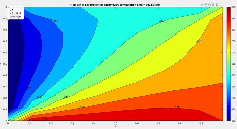
RESULT-
SUCCESIVE OVER RELAXATION-
clear all
close all
clc
%Solving the steady state 2D heat conduction
%sor method(explicit)

%inputs
L=1;
%Number of nodes along x and y diretion
nx=10;
ny=nx;
nt=1400
alpha = 1.2
omega = 1.1

%change of x w.r.t x coordinate
dx=L/(nx-1);
%change of x w.r.t x coordinate
dy=L/(ny-1);

x=linspace(0,1,nx)
y=linspace(0,1,ny);

%defining boundary condition
T_L = 400;
T_T = 600;
T_R = 800;
T_B = 900;
%Temperature array
T = 300*ones(nx,ny);

%Updating the value of temperature
T(2:ny - 1,1) = T_L;
T(2:ny - 1,nx) = T_R;
T(1,2:nx-1) = T_T;
T(ny,2:nx-1) = T_B;

% Calculating the avg temperature at cornors
T(1,1) = (T_T + T_L)/2;
T(nx,ny) = (T_R + T_B)/2;
T(1,ny) = (T_T + T_R)/2;
T(nx,1) = (T_L + T_B)/2;

iterative_solver = 3;
error = 9e9;
tol = 1e-4;
dt =  1e-3

%Assigning the original value to T
T_intial = T;
T_old = T;
T_end = T;

% CFL numbers
k1 = (alpha*dt)/dx^2;
k2 = (alpha*dt)/dy^2;


%SOR method(explicit)
tic;
sor_iteration = 1;

for k = 1:nt
    error = 9e9;

    while(error>tol)

        for i = 2:nx-1

            for j = 2:ny-1
                term1 = 1/(1+(2*k1)+(2*k2));
                term2 = k1*term1
                term3 = k2*term1
                H = (T(i-1,j)) + (T_old(i+1,j))
                V = (T(i,j+1)) + (T_old(i,j-1))

                T(i,j) = (T_intial(i,j)*term1) +(H*term2) + (V*term3)
                T_end(i,j) = ((1-omega)*T_old(i,j)) + (T(i,j)*omega);
            end
        end

        error = max(max(abs(T_old-T)));
        T_old = T_end;
        sor_iteration = sor_iteration+1
    end
    T_intial = T_end;

F = toc;
%ploting the figure
figure(1)
contourf(x,y,T)
clabel(contourf(x,y,T))
colorbar
colormap("jet")
set(gca,'ydir', 'reverse')
xlabel('X')
ylabel('Y')
title(sprintf('Number of sor itration(implicit)=%d,computation time = %f',sor_iteration,F));
pause(0.03)
end
RESULT-
EXPLICIT SCEME -UNSTEADY/TRANSIENT STATE
clear all
close all
clc
%Solving the steady state 2D heat conduction
%sor method(explicit)

%inputs
L=1;
%Number of nodes along x and y diretion
nx=10;
ny=nx;
nt=1400
alpha = 1.2


%change of x w.r.t x coordinate
dx=L/(nx-1);
%change of x w.r.t x coordinate
dy=L/(ny-1);

x=linspace(0,1,nx)
y=linspace(0,1,ny);

%defining boundary condition
T_L = 400;
T_T = 600;
T_R = 800;
T_B = 900;
%Temperature array
T = 300*ones(nx,ny);

%Updating the value of temperature
T(2:ny - 1,1) = T_L;
T(2:ny - 1,nx) = T_R;
T(1,2:nx-1) = T_T;
T(ny,2:nx-1) = T_B;

% Calculating the avg temperature at cornors
T(1,1) = (T_T + T_L)/2;
T(nx,ny) = (T_R + T_B)/2;
T(1,ny) = (T_T + T_R)/2;
T(nx,1) = (T_L + T_B)/2;


error = 9e9;
tol = 1e-4;
dt =  1e-3;
omega = 1.1

%Assigning the original value to T
T_intial = T;
T_old = T;

% CFL numbers
k1 = (alpha*dt)/dx^2;
k2 = (alpha*dt)/dy^2;
iterative_solver = 1


%(explicit)
tic;
if iterative_solver ==1
    stedy_ex = 1;
    for k = 1:nt
        error = 1;
        while(error>tol)
            for i = 2:nx -1;
                for j = 2:ny-1
                    term1 = T_old(i,j);
                    term2 = k1*(T_old(i+1,j) - 2*T_old(i,j) + (T_old(i-1,j)));
                    term3 = k2*(T_old(i,j+1) - 2*T_old(i,j) + (T_old(i,j-1)));
                    T(i,j) = term1 + term2 + term3
                end
            end
            error = max(max(abs(T_old-T)));
            T_old = T;
            stedy_ex = stedy_ex+1
        end
    end
end

F = toc;
%ploting the figure
figure(1)
contourf(x,y,T)
clabel(contourf(x,y,T))
colorbar
colormap("jet")
set(gca,'ydir', 'reverse')
xlabel('X')
ylabel('Y')
title(sprintf('Number of stedy iteration (explicit)=%d,computation time = %f',stedy_ex,F));
pause(0.03)
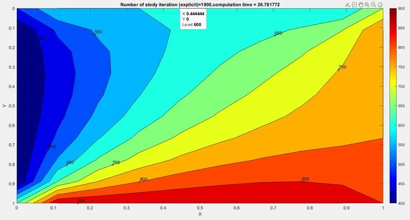
RESULT-
UNSTEADY STATE RESULT-
TYPES OF SCHEMES ITERATION NUMBER COMPUTION TIME
JACOBI 3801 476.25
GAUSS-SEDEL 3532 370.32
SUCCESIVE OVER RELAXATION 3236 390.52
EXPLICT SCHEMS 1900 26.78
CONCLUSION-
From the above results using various iteration method we know the jacobi ,gs and sor are computable in all the scheme and the steady state is more succesfull and less time consuming than unsteady /transient method.