Week 5.1 - Mid term project - Solving the steady and unsteady 2D heat conduction problem
- Steady-state analysis
Solving the 2D state heat conduction equation by using the point interative technique. The boundary is given as follows:
Top boundary layer: 600K
Bottom boundary layer: 900K
Left boundary: 400K
Right boundary: 800K
Solving the steady state implicit equation by using following 3 methods:
- Jacobi
- Gauss-seidel
- Successive over-relaxation
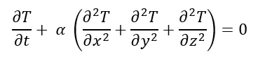
The 3D transient heat conduction equation is given by:
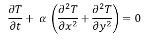
The 2D state form the equation is given as
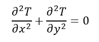
The steady-state form is given as
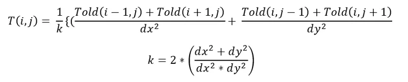
Solving this equation further we get the following equation
clear all
close all
clc

%inputs
nx = 10;
ny = 10;
x = linspace(0,1,nx);
y = linspace(0,1,ny);
dx = x(2)-x(1);
dy = y(2)-y(1);

%[xx,yy] = meshgrid(x,y);
error = 9e9;
tol = 1e-4;

%boundary conditions
T = 300*ones(nx,ny);
T(1,:) = 900;
T(end,:) = 600;
T(:,1) = 400;
T(:,end) = 800;
Told = T;
K = 2*(dx^2+dy^2)/(dx^2*dy^2);

iterative_solver = input('Enter desired  number:');

if iterative_solver==1
    T_Jacobi = jacobi_iter(error,tol,x,y,nx,ny,dx,dy,Told,T,K);
elseif iterative_solver==2
        T_Gauss = gauss_iter(error,tol,x,y,nx,ny,dx,dy,Told,T,K);
    elseif iterative_solver==3
            T_Sor = sor_iter(error,tol,x,y,nx,ny,dx,dy,Told,T,K);
end
function T = jacobi_iter(error,tol,x,y,nx,ny,dx,dy,Told,T,K)
jacobi_iter = 1;
while (error>tol)
for i = 2:nx-1
for j = 2:ny-1
term1 = (Told(i-1,j)+Told(i+1,j))/(K*(dx^2));
term2 = (Told(i,j-1)+Told(i,j+1))/(K*(dy^2));
T(i,j) = term1 + term2;
end
end
error = max(max(abs(Told - T)));
Told = T;
jacobi_iter = jacobi_iter + 1;
figure(1)
contourf(x,y,T)
clabel(contourf(x,y,T));
xlabel('X Axis');
ylabel('Y Axis');
title_txt = sprintf('iteration number = %d',jacobi_iter);
title(title_txt)
pause(0.03)
end
endfunction T = gauss_iter(error,tol,x,y,nx,ny,dx,dy,Told,T,K)
gauss_iteration = 1;
while (error>tol)
for i = 2:nx-1
for j = 2:ny-1
T(i,j) = (((T(i-1,j)+Told(i+1,j))/dx^2)+((T(i,j-1)+Told(i,j+1))/dy^2))/K;
end
end
error = max(max(abs(Told - T)));
Told = T;
gauss_iteration = gauss_iteration + 1;
end
figure(2)
contourf(x,y,T)
clabel(contourf(x,y,T));
xlabel('X Axis');
ylabel('Y Axis');
title_txt = sprintf('iteration number = %d',gauss_iteration);
title(title_txt)
pause(0.03)
end
function T = sor_iter(error,tol,x,y,nx,ny,dx,dy,Told,T,K)
sor_itern = 1;
alpha = 1.7;
while (error>tol)
        for i = 2:nx-1
            for j = 2:ny-1
                S = (((T(i-1,j)+Told(i+1,j))/dx^2)+((T(i,j-1)+Told(i,j+1))/dy^2))/K;
                T(i,j) = alpha*(S)+(1-alpha)*(Told(i,j));
            end
        end
         error = max(max(abs(Told - T)));
         Told = T;
         sor_itern = sor_itern + 1;
figure(3)
contourf(x,y,T)
clabel(contourf(x,y,T));
xlabel('X Axis');
ylabel('Y Axis');
title_txt = sprintf('iteration number = %d',sor_itern);
title(title_txt)
pause(0.03)
end
end
OUTPUT
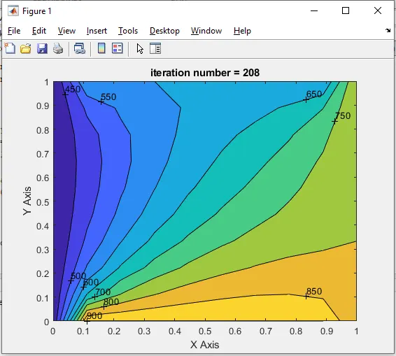
Jacobi:
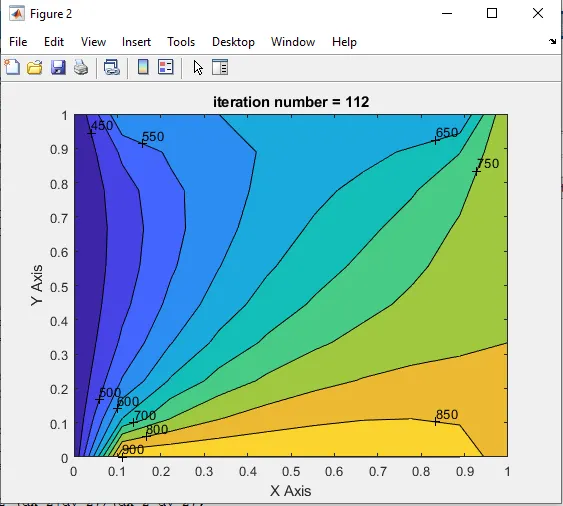
Gauss-seidel
Successive over-relaxation
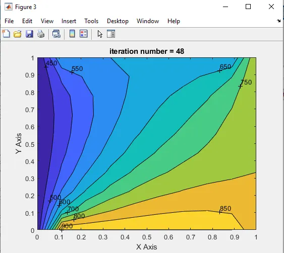
If we compared the output of all the 3 methods Successive over-relaxation takes less time to converge the solution as compared to Jacobi and Gauss-seidel. Hence the SOR method is better than the two.
Solving for Transient Equation:
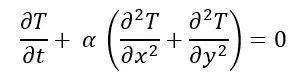
the Transient 2D state equation is given as:
Explicit and implicit methods are used in numerical analysis for obtaining numerical approximations to the solutions of time-dependent (ordinary and partial differential equations), as is required in compute simulations of physical processes.
Explicit methods calculate the state of a system at a later time from the state of the system at the current time, while implicit methods find a solution by solving an equation involving both the current state of the system and the later one.
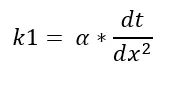
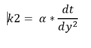
Solving the transient state equation explicitly:

clear all
close all
clc

%inputs
nx = 10;
ny = 10;
x = linspace(0,1,nx);
y = linspace(0,1,ny);
dx = x(2)-x(1);
dy = y(2)-y(1);
dt = 0.01;
alpha = 0.3; %thermal diffusivity

%[xx,yy] = meshgrid(x,y);
%error = 9e9;
%tol = 1e-4;

%boundary conditions
T = 300*ones(nx,ny);
T(1,:) = 900;
T(end,:) = 600;
T(:,1) = 400;
T(:,end) = 800;

%calculating temperature values at the corners
T(1,1) = (400+900)/2;
T(1,ny) = (900+800)/2;
T(nx,1) = (400+600)/2;
T(nx,ny) = (600+800)/2;

Told = T;
K1 = alpha*(dt/dx^2);
K2 = alpha*(dt/dy^2);
iterative_solver = 1;

if iterative_solver==1
T_Jacobi = jacobi_iter_explicit(x,y,nx,ny,Told,T,K1,K2);
end
function T = jacobi_iter_explicit(x,y,nx,ny,Told,T,K1,K2)
jacobi_iter = 1;
for k = 1:300
for i = 2:nx-1
for j = 2:ny-1
term1 = Told(i,j);
term2 = K1*(Told(i+1,j)-2*Told(i,j)+Told(i-1,j));
term3 = K2*(Told(i,j+1)-2*Told(i,j)+Told(i,j-1));
T(i,j) = term1 + term2 + term3;
end
end
%error = max(max(abs(Told - T)));
Told = T;
jacobi_iter = jacobi_iter + 1;
figure(1)
contourf(x,y,T)
clabel(contourf(x,y,T));
xlabel('X Axis');
ylabel('Y Axis');
title_txt = sprintf('iteration number = %d',jacobi_iter);
title(title_txt)
pause(0.03)
end
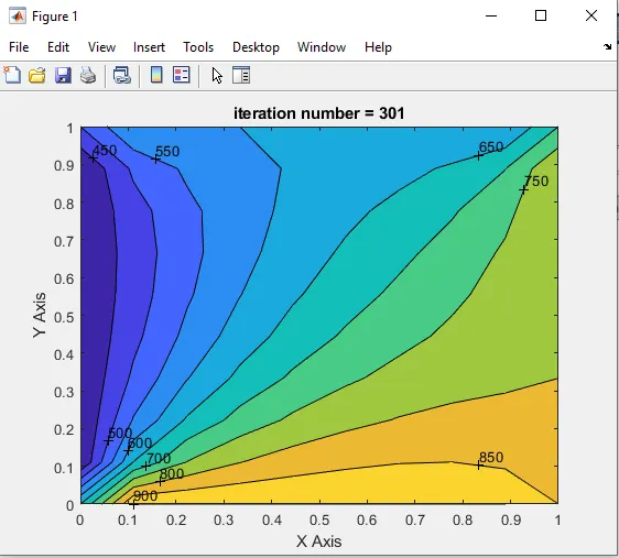
endOUTPUT:
Solving by Implicit method:
While solving the equation by the implicit method. it uses the current state of the steady equation and also the latter one. Technically if Y(t) is the current system state and Y(T+dt) is the state at the later time dt then Y(T+dt) = F(Y(t))
2D heat conduction equation in the implicit form is Given as follows

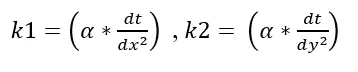
In the Jacobi method, the right-hand side unknown values are assumed that is Tn+1 at all nodes are assumed and hence using the same the LHS is calculated. In the first iteration, the value of T at n+1 is calculated at all nodes, the difference between T at n+1 is obtained. If the value is greater than the specified tolerance value, the iterations are carried out to calculate T at n+1. In the second iteration, the value of T at n+1is assumed as the value of T which was obtained in the previous iteration
Once the value to T is found out iteratively whose error is less than the tolerance value, the value of T is calculated at the next time step n+2 using the same method
The only difference between Gauss Siedel and Jacobi is that when the value of T is calculated at the first node, the updated value at that node is used to calculate at the next node
SOR method can be applied using Jacobi or Gaus Siedel, the only difference has been the addition of new value omega which makes the process faster hence decreasing the number of iteration
CODE:
clear all
close all
clc

nx = 10;
ny = 10;
x = linspace(0,1,nx);
y = linspace(0,1,ny);
dx = x(2)-x(1);
dy = y(2)-y(1);
dt = 0.01;
alpha = 0.3; %thermal diffusivity

%[xx,yy] = meshgrid(x,y);
error = 9e9;
tol = 1e-4;

%boundary conditions
T = 300*ones(nx,ny);
T(1,:) = 900;
T(end,:) = 600;
T(:,1) = 400;
T(:,end) = 800;

%calculating temperature values at the corners
T(1,1) = (400+900)/2;
T(1,ny) = (900+800)/2;
T(nx,1) = (400+600)/2;
T(nx,ny) = (600+800)/2;

Told = T;
tprev_dt = Told;

K1 = alpha*(dt/dx^2);
K2 = alpha*(dt/dy^2);

iterative_solver = input('Enter desired  number:');

if iterative_solver==1
    T_Jacobi = jacobi_iter_implicit(error,tol,x,y,nx,ny,Told,T,tprev_dt,K1,K2);
elseif iterative_solver==2
        T_Gauss = gauss_iter_implicit(error,tol,x,y,nx,ny,Told,T,tprev_dt,K1,K2);
    elseif iterative_solver==3
            T_Sor = sor_iter_implicit(error,tol,x,y,nx,ny,Told,T,tprev_dt,K1,K2);
end
function T = jacobi_iter_implicit(error,tol,x,y,nx,ny,Told,T,tprev_dt,K1,K2)
jacobi_iter = 1;
for p = 1:300
    error=9e9;
    while (error>tol)
        for i = 2:nx-1
            for j = 2:ny-1
                %term1 = (1+(2*K1)+(2*K2)^-1);
                term1 = (1+(2*K1)+(2*K2))^-1;
                term2 = K1*term1;
                term3 = K2*term1;
                h = (Told(i+1,j)+Told(i-1,j));
                v = (Told(i,j+1)+Told(i,j-1));
                T(i,j) = ((tprev_dt(i,j)*term1)+(h*term2)+(v*term3));
            end
        end
         error = max(max(abs(Told - T)));
         Told = T;
         jacobi_iter = jacobi_iter + 1;
    end
    tprev_dt = T;
end
figure(1)
contourf(x,y,T)
clabel(contourf(x,y,T));
xlabel('X Axis');
ylabel('Y Axis');
title_txt = sprintf('iteration number = %d',jacobi_iter);
title(title_txt)
pause(0.03)
end
function T = gauss_iter_implicit(error,tol,x,y,nx,ny,Told,T,tprev_dt,K1,K2)
gauss_iteration = 1;
for p = 1:300
error=9e9;
while (error>tol)
for i = 2:nx-1
for j = 2:ny-1
%term1 = (1+(2*K1)+(2*K2)^-1);
term1 = (1+(2*K1)+(2*K2))^-1;
term2 = K1*term1;
term3 = K2*term1;
h = (T(i+1,j)+Told(i-1,j));
v = (Told(i,j+1)+Told(i,j-1));
T(i,j) = ((tprev_dt(i,j)*term1)+(h*term2)+(v*term3));
end
end
error = max(max(abs(Told - T)));
Told = T;
gauss_iteration = gauss_iteration + 1;
end
tprev_dt = T;
end
figure(2)
contourf(x,y,T)
clabel(contourf(x,y,T));
xlabel('X Axis');
ylabel('Y Axis');
title_txt = sprintf('iteration number = %d',gauss_iteration);
title(title_txt)
pause(0.03)
end
function T = sor_iter_implicit(error,tol,x,y,nx,ny,Told,T,tprev_dt,K1,K2)
sor_itern = 1;
omega = 1.2;
for  p = 1:300
    error=9e9;
    while (error>tol)
        for i = 2:nx-1
            for j = 2:ny-1
                %term1 = (1+(2*K1)+(2*K2)^-1);
                term1 = (1+(2*K1)+(2*K2))^-1;
                term2 = K1*term1;
                term3 = K2*term1;
                h = (T(i+1,j)+Told(i-1,j));
                v = (Told(i,j+1)+Told(i,j-1));
                T(i,j) = (Told(i,j)*(1-omega))+(omega*((tprev_dt(i,j)*term1)+(h*term2)+(v*term3)));
            end
        end
         error = max(max(abs(Told - T)));
         Told = T;
         sor_itern = sor_itern + 1;
    end
    tprev_dt = T;
end
figure(3)
contourf(x,y,T)
clabel(contourf(x,y,T));
xlabel('X Axis');
ylabel('Y Axis');
title_txt = sprintf('iteration number = %d',sor_itern);
title(title_txt)
pause(0.03)
end
OUTPUT:
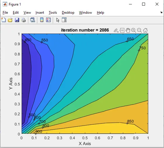
Jacobi
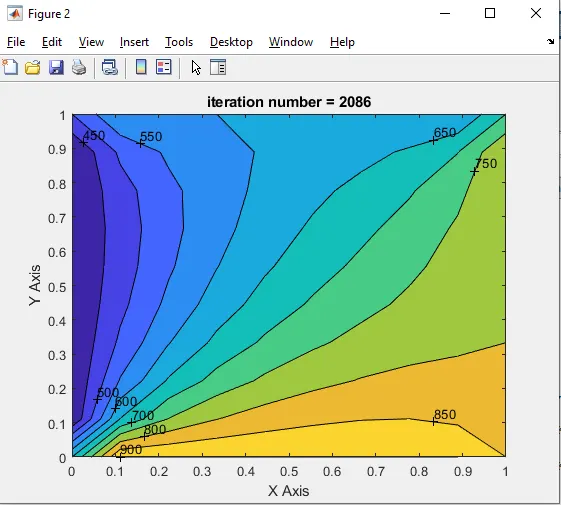
Gauss Siedal
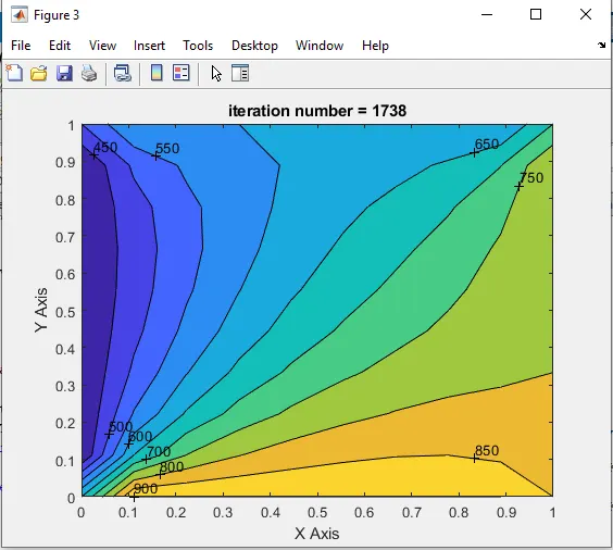
SOR
Conclusion:
Based on various methods used to solve the steady-state equation is it clear that the time SOR method gives the results very fast with less amount iteration and time as compared to Jacobi and Gauss Siedel.
whereas the time required to solve the transient equation is way more as compared to steady-state
when solving the Explicit method for transient equations it yields results very fast since all the values are already known to us. but this can be only be done if the CFL is less than 0.25
Eben while solving the transient equation implicitly the number of iterations taken to solve the solution by Jacobi and Gauss Siedel is more as compared to SOR
Since the addition of extra terms like alpha(thermal diffusivity) and also the time derivative the time required for convergence is more