Week 3 - Solving second order ODEs

A second-order differential equation is very important in the field of physics and engineering, which helps us to know different phenomenon of it wherein we often have to find the functions of function which satisfy out differential equation. These equations work for different systems related to engineering like pendulum, spring-mass-damper system which are very useful in the field of vibrations, resistor-inductor-capacitor connected in series.

Aim: To solve the following differential equation of a simple pendulum and plot the graph and the animate the process.

Procedure:

• To plot displacement and velocity plots with respect to time. In this type of solution, we have used a different function called ode45 which uses ode function, time, and initial condition. the following code is represented and follows and the output is attached below along with ode function code.

clear all
close all
clc

%inputs
b = 0.05;
g = 9.81;
L = 1;
m = 1;


%initial condition
theta = [0;3];

%time
time = linspace(0,20,200);

%solution
[t,result] = ode45(@(t,theta) ode_func(t,theta,b,g,L,m),time,theta);

plot(t,result(:,1),'color','b')
hold on
plot(t,result(:,2),'color','r')
xlabel('time')
ylabel('plot')

function [dtheta_dt] = ode_func(t,theta,b,g,L,m)
theta1=theta(1)
theta2=theta(2)
dtheta1_dt = theta2;
dtheta2_dt = -(b/m)*theta2-(g/L)*sin(theta1);
dtheta_dt = [dtheta1_dt;dtheta2_dt];
end

• Output

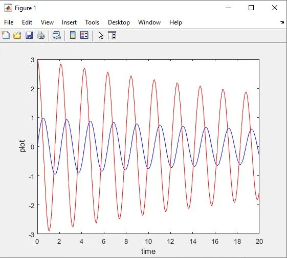
• To animate the video of working of a pendulum wherein one is fixed and the other end moves with respect to the ode function that we have solved.

clear all
close all
clc

%inputs
b = 0.05;
g = 9.81;
L = 1;
m = 1;


%initial condition
theta = [0;3];

%time
time = linspace(0,20,200);

%solution
[t,result] = ode45(@(t,theta) ode_func(t,theta,b,g,L,m),time,theta);

ct = 1;
for i = 1:length(result(:,1))
    x0 = 0;
    y0 = 0;
    x1 = L*sin(result(i,1));
    y1 = -L*cos(result(i,1));
    plot([-1 1],[0 0],'linewidth',2,'color','b');
    hold on
    line([x0 x1],[y0 y1],'linewidth',2,'color','r');
    hold on
    plot(x1,y1,'o','markers',20,'markerfacecolor','y');
    grid on
    axis([-1.5 1.5 -1.5 0.5])
    pause(0.03)
    hold off
    M(ct) = getframe(gcf)
    ct = ct+1;
end

movie(M)
videofile = VideoWriter('Pendulum.avi','Uncompressed avi');
open(videofile)
writeVideo(videofile,M)
close