Week 3.5 - Deriving 4th order approximation of a 2nd order derivative using Taylor Table method

Aim: To derive the fourth-order approximation of the second-order derivative using the central differencing method, skewed right-sided difference, and skewed left-sided difference:

Consider the second-order function:

1. Central differencing

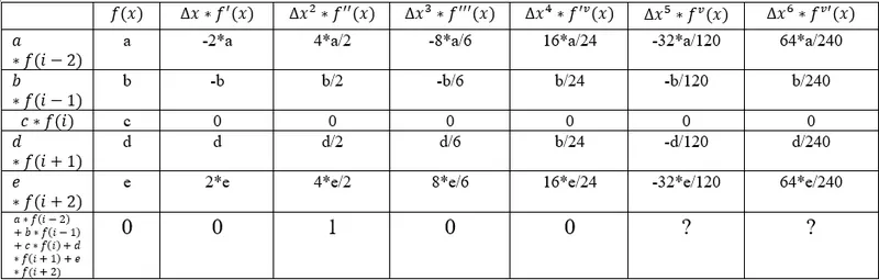
For the third column, the sum is one because we are computing 2^nd order derivative.

If we take our function, we're basically having only 5 terms which mean technically only for the first five terms we know that which of the column will sum to zero. Also, we only have 5 equations to solve and 5 unknowns. So, if we do add additional equation like column 5 and 6 and accidentally put zero then we are over-specifying the system and hence that term is not zero

Converting the table into matrix form:

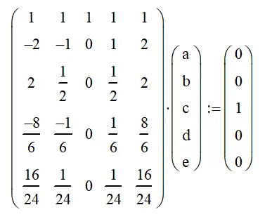
A = [ 1 1 1 1 1 ; -2 -1 0 1 2 ; 2 ½ 0 ½ 2 ; -8/6 -1/6 0 1/6 8/6 ; 16/24 1/24 0 1/24 16/24];

B = [0;0;1;0;0];

X = A\B;

X = (a = -0.0833, b = 1.3333, c = 0, d = 1.3333, e = -0.0833)

We can conclude from it that a = e, b = d.

2. Skewed right-sided difference

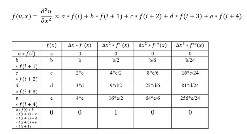
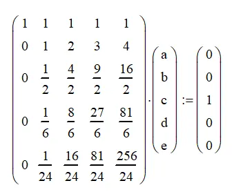
After evaluating we get

a = 0.9188, b = -1.4744, c = -0.0897, d = 0.9274, e = -0.2821

3. Skewed left-sided difference

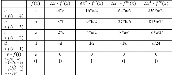
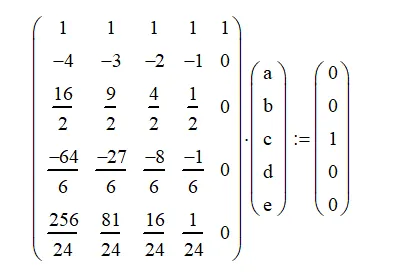
After evaluation values are

a = 0.9167, b = -4.6667, c = 9.5, d = -8.6667, e = 2.9167

Now writing a program in Matlab to evaluate the second-order derivative of the analytical function exp(x)*cos(x) and to compare it with the 3 numerical approximations that we have derived above.

our first task in writing the program is to derive the coefficient of 4th order approximation of second-order derivative for central differencing, skewed right side difference, and skewed left side difference after that writing the program to determine the truncation error for all the three differencing after which we define the for loop for the number of iterations to be performed and writing the functions for calculating truncation error for central differencing, skewed right side difference and skewed left side difference.

once the error is calculated we plot the graphs to evaluate the truncation error.

clear all
close all
clc

%getting coefficient through central differecing method
A = [ 1 1 1 1 1;-2 -1 0 1 2;2 1/2 0 1/2 2;-8/6 -1/6 0 1/6 8/6;16/24 1/24 0 1/24 16/24];
B = [0;0;1;0;0];
X = A\B;

%getting coefficient through skewed right side difference method
C = [1 1 1 1 1;0 1 2 3 4;0 1/2 4/2 9/2 16/2;0 1/6 8/6 27/6 64/6;0 1/24 16/24 81/24 256/24];
D = [0;0;1;0;0];
Y = C\D;

%getting coefficient through skewed left side differecing method
E = [1 1 1 1 1;-4 -3 -2 -1 0;16/2 9/2 4/2 1/2 0;-64/6 -27/6 -8/6 -1/6 0;256/24 81/24 16/24 1/24 0];
F = [0;0;1;0;0];
Z = E\F;

x = pi/3;
dx = linspace(pi/30,pi/300,20);

%given function
f = exp(x)*cos(x);

%analytical derivative
ad = -2*exp(x)*sin(x);

for i = 1:length(dx)
    cd_error(i) = central_difference(x,dx(i),X);
    sr_error(i) = skewed_right_error(x,dx(i),Y);
    sl_error(i) = skewed_left_error(x,dx(i),Z);
end

figure(1)
loglog(dx,cd_error,'linewidth',2,'color','r');
hold on
loglog(dx,sr_error,'linewidth',2,'color','b');
hold on 
loglog(dx,sl_error,'linewidth',2,'color','y');
legend('central difference','skewed right-side difference','skewed lift-sided difference','location','northwest');
xlabel('dx(grid-size)');
ylabel('truncation_error');

function out = central_difference(x,dx,X)
f1 = exp(x-2*dx)*cos(x-2*dx);
f2 = exp(x-1*dx)*cos(x-1*dx);
f3 = exp(x)*cos(x);
f4 = exp(x+1*dx)*cos(x+1*dx);
f5 = exp(x+2*dx)*cos(x+2*dx);
ad = -2*exp(x)*sin(x);
cent_diff = (X(1)*f1+X(2)*f2+X(3)*f3+X(4)*f4+X(5)*f5)/(dx^2);
out = abs(cent_diff - ad);
end

function out = skewed_right_error(x,dx,Y)
f6 = exp(x)*cos(x);
f7 =exp(x+1*dx)*cos(x+1*dx);
f8 =exp(x+2*dx)*cos(x+2*dx);
f9 =exp(x+3*dx)*cos(x+3*dx);
f10 =exp(x+4*dx)*cos(x+4*dx);
ad = -2*exp(x)*sin(x);
skewed_right = (Y(1)*f6+Y(2)*f7+Y(3)*f8+Y(4)*f9+Y(5)*f10)/(dx^2);
out = abs(skewed_right - ad);
end

function out = skewed_left_error(x,dx,Z)
f11 = exp(x-4*dx)*cos(x-4*dx);
f12 =exp(x-3*dx)*cos(x-3*dx);
f13 =exp(x-2*dx)*cos(x-2*dx);
f14 =exp(x-1*dx)*cos(x-1*dx);
f15 =exp(x)*cos(x);
ad = -2*exp(x)*sin(x);
skewed_left = (Z(1)*f11+Z(2)*f12+Z(3)*f13+Z(4)*f14+Z(5)*f15)/(dx^2);
out = abs(skewed_left - ad);
end

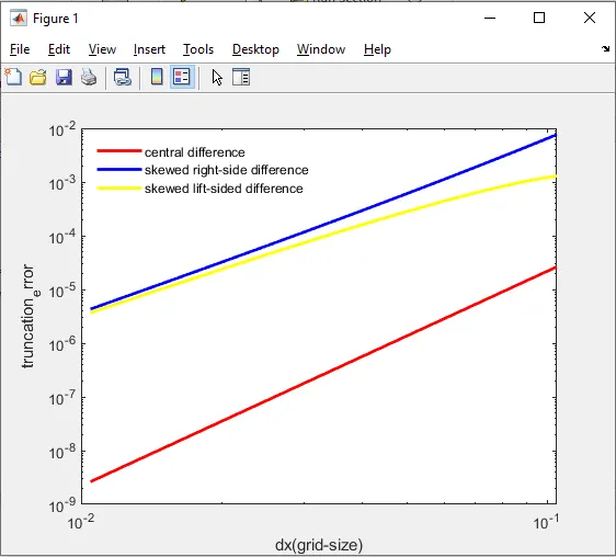
As we can observe from the above graph that the truncations error for 4th order approximation for second-order derivative through central differencing is very low compared to the skewed right side and skewed left side differencing and this is mainly because the central differencing considers values from both sides of the grid point, therefore, central differencing is a good numerical approximation.