Week 4 - Genetic Algorithm
Optimization
Optimization is a selection process which helps us to find the best results or solution of the given function under certain criteria or limitation. Basically, in this process, various solutions outcomes are compared with each other, and an optimal solution is selected.
For example, if you want to get to destination ‘A’ from ‘B’ and you have various paths to reach your destination optimization process will help you figure out which path is more convenient for you to travel and will save your time as well.
To carry out the optimization process various variables and constraints are taken into consideration. Variables are those parameters that will keep on changing when the optimization process is been carried out and constraints are used to make sure our output doesn’t go beyond a certain desired limit.
Genetic Algorithm
To carry out the optimization there are various algorithms and a genetic algorithm is one of them. The genetic algorithm is based on the principle of genetics and selection process which either gives us an exact optimal solution or close to actual solution results.
Once the program starts running the algorithm the randomness of the population is initialized then the fitness of the function is calculated and the optional solution is found if not then as per the principles of genetics mutation, selection and crossover is carried out and the result is again transferred to calculate the fitness and the program is terminated.
Syntax for Genetic Algorithm in MATLAB
x = ga(fun,nvars,A,b,Aeq,beq,lb,ub)
x = ga(fun,nvars,A,b,Aeq,beq,lb,ub,nonlcon)
x = ga(fun,nvars,A,b,Aeq,beq,lb,ub,nonlcon,options)
x = ga(fun,nvars,A,b,[],[],lb,ub,nonlcon,IntCon)
x = ga(fun,nvars,A,b,[],[],lb,ub,nonlcon,IntCon,options)
where,
fun: function
nvars: number of variables
A,b: linear inequality constraints
Aeq, beq: linear equality constraints
lb, ub: lower bound and upper bound
nonlcon: non-linear constraints
options: optimization options
Intcon: integer variables
Aim: Our objective is to find the maxima of the given function
Case 1:
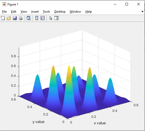
To create a stalagmite function and plot a 3-dimensional plot which shows us local as well as global maxima and for maxima we have added negative sign so that the stalagmite graph is reversed.
function [f] = stalagmite(input_vector)
x = input_vector(1);
y = input_vector(2);

f1x = (sin (5.1*pi*x + 0.5)).^6;
f1y = (sin (5.1*pi*y + 0.5)).^6;

a1 = ((x-0.0667).^2)/(0.64);
f2x = exp(-4.*log(2)*a1);

a2 = ((y-0.0667).^2)/(0.64);
f2y = exp(-4.*log(2)*a2);

f = -(f1x.*f2x.*f1y.*f2y);
end
clear all
close all
clc
x = linspace(0,0.6,150);
y = linspace(0,0.6,150);
[xx,yy] = meshgrid(x,y);
for i = 1:length(xx)
for j = 1:length(yy)
input_vector(1) = xx(i,j);
input_vector(2) = yy(i,j);
f(i,j) = stalagmite(input_vector);
end
end
surfc(xx,yy,-f);
shading interp
xlabel('x value');
ylabel('y value');
[input, fval] = ga(@stalagmite,2)
Output:
Case 2:
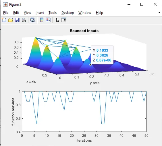
Statistical behavior of the genetic algorithm and use of upper and lower bound
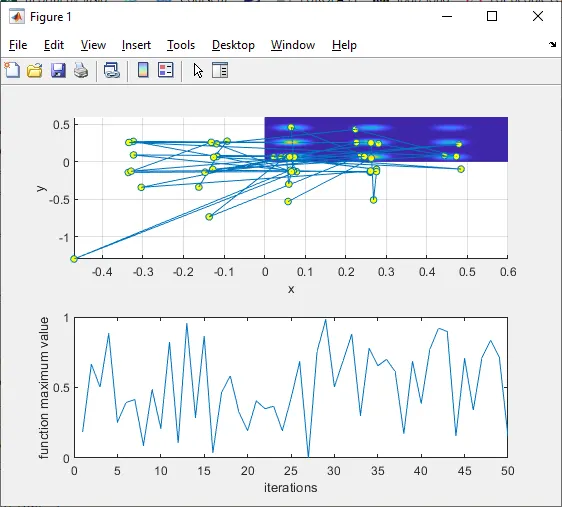
Here the minimum values evaluated by the ga function have scattered all over the plot and that is because of random sampling so each and every time we run the code we will get different results. Since we have provided 50 iterations and we can see that during each iteration the value changes. Hence the result is not usable. To get better results we will set up upper and lower bounds.
As we can see our maximum value is 0 and 1 so we will set the lower bound to [0:0] and the upper bound to [1;1]
clear all
close all
clc

x = linspace(0,0.6,150);
y = linspace(0,0.6,150);
num_case = 50;

[xx,yy] = meshgrid(x,y);

for i = 1:length(xx)
    for j = 1:length(yy)
        input_vector(1) = xx(i,j);
        input_vector(2) = yy(i,j);
        f(i,j) = stalagmite(input_vector);
    end
end

surfc(xx,yy,-f);
shading interp

tic
for i = 1:num_case
    [input,fopt(i)] = ga(@stalagmite,2);
    xopt(i) = input(1);
    yopt(i) = input(2);
end

stuty1_time = toc

figure(1)
subplot(2,1,1);
hold on
surfc(xx,yy,-f);
hold on
shading interp
plot3(xopt,yopt,-fopt,'marker','o','markersize',5,'markerfacecolor','y');
xlabel('x')
ylabel('y')
grid on
subplot(2,1,2)
plot(-fopt);
xlabel('iterations');
ylabel('function maximum value')

%upperbound lowerbound
tic
for i = 1:num_case
    [input,fopt(i)] = ga(@stalagmite,2,[],[],[],[],[0;0],[1;1]);
    xopt(i) = input(1);
    yopt(i) = input(2);
end
study2_time = toc;

figure(2)
subplot(2,1,1)
hold on
surfc(xx,yy,-f)
shading interp
plot3(xopt,yopt,-fopt,'marker','o','markersize',5,'markerfacecolor','y')
xlabel('x axis')
ylabel('y axis')
title('Bounded inputs')
subplot(2,1,2)
plot(-fopt)
xlabel('iterations')
ylabel('function maxima')
Output:
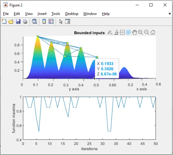
As we can see in the result our result is much narrower than the previous result and our maximum value lies between a certain range.
Case 3:
To increase the population size by increasing the population size we can get our global maxima value and the drawback of this method is that it will take a lot of time to execute the algorithm
clear all
close all
clc

x = linspace(0,0.6,150);
y = linspace(0,0.6,150);
num_case = 50;

[xx,yy] = meshgrid(x,y);

for i = 1:length(xx)
    for j = 1:length(yy)
        input_vector(1) = xx(i,j);
        input_vector(2) = yy(i,j);
        f(i,j) = stalagmite(input_vector);
    end
end

surfc(xx,yy,-f);
shading interp

tic
for i = 1:num_case
    [input,fopt(i)] = ga(@stalagmite,2);
    xopt(i) = input(1);
    yopt(i) = input(2);
end

stuty1_time = toc

figure(1)
subplot(2,1,1);
hold on
surfc(xx,yy,-f);
hold on
shading interp
plot3(xopt,yopt,-fopt,'marker','o','markersize',5,'markerfacecolor','y');
xlabel('x')
ylabel('y')
grid on
subplot(2,1,2)
plot(-fopt);
xlabel('iterations');
ylabel('function maximum value')

%upperbound lowerbound
tic
for i = 1:num_case
    [input,fopt(i)] = ga(@stalagmite,2,[],[],[],[],[0;0],[1;1]);
    xopt(i) = input(1);
    yopt(i) = input(2);
end
study2_time = toc;

figure(2)
subplot(2,1,1)
hold on
surfc(xx,yy,-f)
shading interp
plot3(xopt,yopt,-fopt,'marker','o','markersize',5,'markerfacecolor','y')
xlabel('x axis')
ylabel('y axis')
title('Bounded inputs')
subplot(2,1,2)
plot(-fopt)
xlabel('iterations')
ylabel('function maxima')

%increasing GA iterations
options = optimoptions('ga');
options = optimoptions(options,'populationsize',300);

tic
for i = 1:num_case
[input,fopt(i)] = ga(@stalagmite,2,[],[],[],[],[0;0],[1;1],[],[],options);
    xopt(i) = input(1);
    yopt(i) = input(2);
end
study3_time = toc

figure(3)
subplot(2,1,1)
hold on
surfc(x,y,-f)
shading interp
plot3(xopt,yopt,-fopt,'marker','o','markersize',5,'markerfacecolor','y')
xlabel('x axis')
ylabel('y axis')
title('bounded inputs with increse in population size')
subplot(2,1,2)
plot(-fopt)
xlabel('iterations')
ylabel('function maxima')
output:
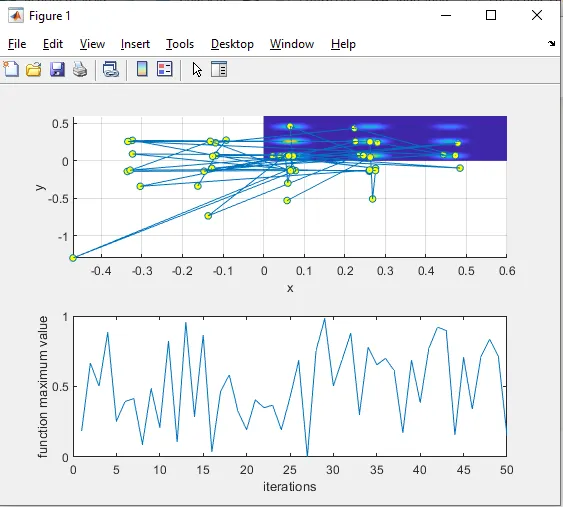
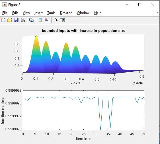
As we can see our maximum values approximately between 0.9999998 and 0.9999999 except for two interactions to get an exact result we can increase our population size but that will also increase our simulation time.