Week 5.1 - Mid term project - Solving the steady and unsteady 2D heat conduction problem
Aim:
To solve 2D heat conduction equation using implicit (poin iterative method) and Explicit schemes.
Description:
2D dimension heat conduction equation is given by `(delT)/(delt)=alpha((del^2T)/(delx^2)+(del^2T)/(dely^2))`
`(delT)/(delt)` is known as time derivative term
`alpha` is thermal diffusivity of the medium
Heat transfer is classified into steady state and transient state (unsteady) heat transfer.
steady state is where the temperature within the system is constant through out the medium, where as in transient state heat transfer the temperature of the system varies with respect to time.
Hence equation can be further obtained for steady and unsteady condition
Equation for ,
Steady state heat transfer is `(del^2T)/(delx^2)+(del^2T)/(dely^2)=0`
Unsteady state heat transfer is `(delT)/(delt)=alpha((del^2T)/(delx^2)+(del^2T)/(dely^2))`
Boundary conditions:
Consider domain as a unit square
Top Boundary = 600 K (K is Kelvin)
Bottom Boundary = 900 K
Left Boundary = 400 K
Right Boundary = 800 K
Lets consider the inner node values as 300K for the time sake. it will affect the iteration or result, over the iterations the value will reach its true value
thermal diffusivity = 1.4 m^2/s
Steady state heat conduction:
1. Discretization:
The steady state 2D heat conduction eqn is given by `(del^2T)/(delx^2)+(del^2T)/(dely^2)=0`
Discretize the above solution using central scheme method
Let consider,
`T_L`=Left node
`T_R`= Right node
`T_P`= Present node
`T_B`= Bottom node
`T_T`= Top node
The discretized equation is given by `(T_L-2T_P+T_R)/(Deltax^2)+(T_T-2T_P+T_B)/(Deltay^2)=0`
Simplifying the above equation,
`T_P=1/k[(T_L+T_R)/(Deltax^2)+(T_T+T_B)/(Deltay^2)]`
Where, `k=2((Deltax^2+Deltay^2)/(Deltax^2Deltay^2))`
Since `Deltax=Deltay` in this case
`T_P=0.25(T_L+T_R+T_T+T_B)`
2.Main Program:
Iterative solvers:
- Jacobi iteration - It uses values updated from the previous step for next iteration and iteration takes place untill the value converges that residual value is less than the required tolerance value
- Gauss seidel iteration - It uses the latest updated values for each iteration until the residual value converges within the limit. Hence it is iterated with the updated values the number of step required to obtain the result will be lesser than the Jacobi method
- Succesive over relaxation iteration - This method is used to speedup either of the two iteration methods which uses a relaxation parameter denoted as `omega`.
The equation is given by `T_p^(n+1)=(1-omega)*T_((gs or j))+omega*T_p^n`
If `0<omega<1` - It is known as under relaxation (slow down the process)
If `1<omega<2` - It is known as over relaxation (speed up the process)
If `omega=1` - It means relaxation cannot be done, Equation simplifies into either jacobi or gauss seidel form.
It is important to choose optimum realxation parameter, else the result would be fluctuating arround the answer leading to time delay and increase in number of iteration involved.
%Solving steady and unsteady 2D heat conduction problem

% *steady state 2D heat conduction problem:*
%Experession is given by
%(\partial^2/\partialx^2)+(\partial^2/\partialy^2)=0
%solving by implicit method using different iterative methods
clear all %#ok
close all
clc
%Initial conditions
nx=10;
ny=nx; %no of grid points
x=linspace(0,1,nx);
y=x;
dx= x(2)-x(1);
dy=dx;
omega=1.5;
%Defining the tol values for result to converge
error = 9e9;
tol=1e-4;

%Boundary condition
T=300*ones(nx,ny); %all initial nodes temp are assumed to be 300k
T(1,2:ny-1)=600;  %Top boundary
T(nx,2:ny-1)=900; %Bottom boundary
T(2:nx-1,1)=400;  %Left boundary
T(2:nx-1,ny)=800; %Right boundary

%Avg temp at corners
T(1,1)= (T(1,2)+T(2,1))/2;
T(1,ny)= (T(1,ny-1)+T(2,ny))/2;
T(nx,1)= (T(nx-1,1)+T(nx,2))/2;
T(nx,ny)= (T(nx-1,ny)+T(nx,ny-1))/2;

T_old=T;

prompt="Please select appropriate iterative solver: \n1-Jacobi iteration\n2-Gauss seidel iteration\n3-Succesive over relaxation iteration\n";
solver=input(prompt);

%Jacobi Iteration method
if solver==1
   j_iter=1;
   while(error>tol)
       for i=2:nx-1
           for j=2:ny-1
               T(i,j)= 0.25*(T_old(i-1,j)+T_old(i+1,j)+T_old(i,j+1)+T_old(i,j-1));
           end
       end
       error= max(max(abs(T_old-T)));
       T_old=T;
       j_iter=j_iter+1;
   end

%Plotting contour graph of temperature distribution
figure(1)
contourf(x,y,T)
clabel(contourf(x,y,T))
colorbar
colormap(jet)
set(gca,'ydir','reverse')

xlabel('X-axis')
ylabel('Y-axis')
title(sprintf('Steady  state: No of Jacobi iteration = %d',j_iter))
pause(0.3)
end

%Gauss seidel Iteration method
if solver==2
   gs_iter=1;
   while(error>tol)
       for i=2:nx-1
           for j=2:ny-1
               T(i,j)= 0.25*(T(i-1,j)+T_old(i+1,j)+T_old(i,j+1)+T(i,j-1));
           end
       end
       error= max(max(abs(T_old-T)));
       T_old=T;
       gs_iter=gs_iter+1;
   end

%Plotting contour graph of temperature distribution
figure(2)
contourf(x,y,T)
clabel(contourf(x,y,T))
colorbar
colormap(jet)
set(gca,'ydir','reverse')

xlabel('X-axis')
ylabel('Y-axis')
title(sprintf('Steady  state: No of Gauss seidel iteration = %d',gs_iter))
pause(0.3)
end

%Succesive over relaxation Iteration method
if solver==3
   sor_iter=1;
   while(error>tol)
       for i=2:nx-1
           for j=2:ny-1
               T(i,j)= omega*(0.25*(T(i-1,j)+T_old(i+1,j)+T_old(i,j+1)+T(i,j-1)))+(1-omega)*T_old(i,j);
           end
       end
       error= max(max(abs(T_old-T)));
       T_old=T;
       sor_iter=sor_iter+1;
   end

%Plotting contour graph of temperature distribution
figure(2)
contourf(x,y,T)
clabel(contourf(x,y,T))
colorbar
colormap(jet)
set(gca,'ydir','reverse')

xlabel('X-axis')
ylabel('Y-axis')
title(sprintf('Steady  state: No of SOR iteration = %d',sor_iter))
pause(0.3)
end
3.Explanation:
- In this program, code has been written to perform iterative solving of 2D heat convectional equation using Jacobi iteration, Gauss seidel iteration and Succesive over relaxation iteration
- While compling the code, compiler request for user input for selecting either of the iteration method
- once the input is given, if loop is used to select appropriate iteration to be done
- Plot command has been used along with no of iterations involved to understand the basic method of iterative solvers function in arriving the solution.
4. Plot:
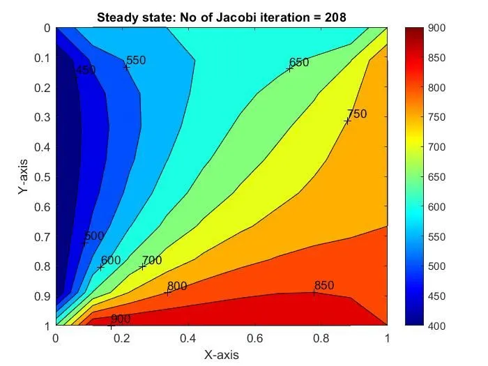
- Jacobi iteration: (for input 1)
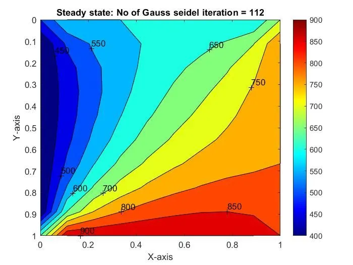
- Guass seidel Iteration:(for input 2)
- Succesive over relaxation iteration:(for input 3)
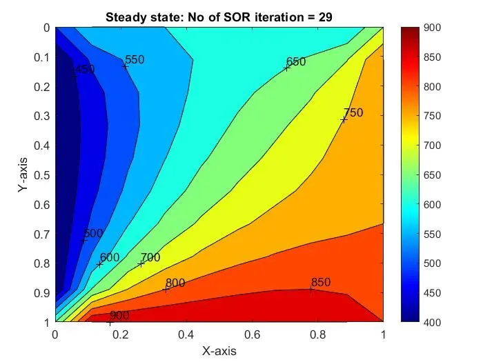
From the above plots and no of iterations for each method, we can understand that no of Jacobi>gauss seidel>SOR iterations.
It clearly shows that, SOR speed up the process of Jacobi and Gauss seidel methods.
Unsteady or transient state condition:
The boundary conditions are used for transient state 2D heat conduction equation.
Since, temperature may vary with respect to time, this would be a time marching problem and we have to define the time step and no. of time steps for solving
let, dt(time step) = 0.02 and nt(no. of time step) = 1400
In time marching solution, we have to focus on CFL number.
Courant number: Courant number is a measure of how much information traverses a computational grid in a given time step.
for 2D heat conduction equation, courant number is mathematically given by, `CFL=alpha(dt/(dx^2))`
`CFL`=Courant Friedrichs Lewy conndition or Courant number
`alpha`= Thermal diffusivity (m^2/s)
`dt`= time step (s)
`dx`= grid space (m)
In this case, the CFL number should be below 0.5 for Explit method of solving the equation else the solution woul blow up
i.e `CFL_x+CFL_y<=0.5`
For implicit solution, this criteria wont be needed since it is unconditionaly stable.
1. Discretization:
The unsteady state 2D heat conduction eqn is given by `(delT)/(delt)=alpha((del^2T)/(delx^2)+(del^2T)/(dely^2))`
Discretize the above solution using central scheme method for spacial terms and forward scheme for time derivative
Let consider,
`T_L`=Left node
`T_R`= Right node
`T_P`= Present node
`T_B`= Bottom node
`T_T`= Top node
The discretized equation is given by
for Explicit method,
`(T_p^(n+1)-T_p^(n))/(Deltat)=alpha*((T_L-2T_P+T_R)/(Deltax^2)+(T_T-2T_P+T_B)/(Deltay^2))^n`
simplifying the above equation,
`T_p^(n+1)=T_p^n+k_1(T_L-2T_P+T_R)^n+k_2(T_T-2T_P+T_B)^n`
where, `k_1=alpha.(delt)/(delx^2)`
`k_2=alpha.(delt)/(dely^2)`
For implicit method,
`(T_p^(n+1)-T_p^(n))/(Deltat)=alpha*((T_L-2T_P+T_R)/(Deltax^2)+(T_T-2T_P+T_B)/(Deltay^2))^(n+1)`
Simplifying the above equation,
`T_p^(n+1)=T_p^n/(1+2k_1+2k_2)+k_1/(1+2k_1+2k_2)*(T_L+T_R)^(n+1)+k_2/(1+2k_1+2k_2)*(T_T+T_B)^(n+1)`
where, `k_1=alpha.(delt)/(delx^2)`
`k_2=alpha.(delt)/(dely^2)`
2.Main Program:
%Solving steady and unsteady 2D heat conduction problem

% *Unsteady state 2D heat conduction problem:*
%Experession is given by
%(\partialT/\Partialt)-alpha((\partial^2T/\partialx^2)+(\partial^2T/\partialy^2))=0
%solving by explicit and implicit method using different iterative methods
clear all %#ok<CLALL>
close all
clc
%Initial conditions
nx=10;
ny=nx; %no of grid points
x=linspace(0,1,nx);
y=x;
dx= x(2)-x(1);
dy=dx;
nt=1400; %no.of timesteps
omega=1.5; %SOR - relaxation parameter
alpha=1.4; % thermal diffusivity
dt=0.002; %time step

%Defining the tolerance values for result to converge

tol=1e-4;

%Boundary condition
T=300*ones(nx,ny); %all initial inner nodes temp are assumed to be 300k
T(1,2:ny-1)=600;  %Top boundary
T(nx,2:ny-1)=900; %Bottom boundary
T(2:nx-1,1)=400;  %Left boundary
T(2:nx-1,ny)=800; %Right boundary

%Avg temp at corners
T(1,1)= (T(1,2)+T(2,1))/2;
T(1,ny)= (T(1,ny-1)+T(2,ny))/2;
T(nx,1)= (T(nx-1,1)+T(nx,2))/2;
T(nx,ny)= (T(nx-1,ny)+T(nx,ny-1))/2;

T_old=T;
T_prev=T;
k1=(alpha*dt)/(dx^2);
k2=(alpha*dt)/(dy^2);

prompt="Please select appropriate iterative solver: \n1-Jacobi iteration\n2-Gauss seidel iteration\n3-Succesive over relaxation iteration\n4-Explicit method\n";
solver=input(prompt);

%Jacobi Iteration method
if solver==1
   j_iter=1;
   for a=1:nt % time loop
   error = 9e9;
    while(error>tol) %converge loop
       for i=2:nx-1
           for j=2:ny-1
               term1=(1+2*k1+2*k2)^(-1);
               term2=k1*term1*(T_old(i-1,j)+T_old(i+1,j));
               term3=k2*term1*(T_old(i,j+1)+T_old(i,j-1));
               T(i,j)= T_prev(i,j)*term1+term2+term3;
           end
       end
       error= max(max(abs(T_old-T)));
       T_old=T;
       j_iter=j_iter+1;
    end
T_prev=T;
   end
%Plotting contour graph of temperature distribution
figure(1)
contourf(x,y,T)
clabel(contourf(x,y,T))
colorbar
colormap(jet)
set(gca,'ydir','reverse')

xlabel('X-axis')
ylabel('Y-axis')
title(sprintf('Unsteady state: No of Jacobi iteration = %d',j_iter))
end


%Gauss seidel Iteration method
if solver==2
   gs_iter=1;
  for a=1:nt % time loop
  error = 9e9;
   while(error>tol)
       for i=2:nx-1
           for j=2:ny-1
               term1=(1+2*k1+2*k2)^-1;
               term2=k1*term1*(T(i-1,j)+T_old(i+1,j));
               term3=k2*term1*(T_old(i,j+1)+T(i,j-1));
               T(i,j)= T_prev(i,j)*term1+term2+term3;
           end
       end
       error= max(max(abs(T_old-T)));
       T_old=T;
       gs_iter=gs_iter+1;
   end
T_prev=T;
  end
%Plotting contour graph of temperature distribution
figure(2)
contourf(x,y,T)
clabel(contourf(x,y,T))
colorbar
colormap(jet)
set(gca,'ydir','reverse')

xlabel('X-axis')
ylabel('Y-axis')
title(sprintf('Unsteady state: No of Gauss seidel iteration = %d',gs_iter))
pause(0.3)
end

%Succesive over relaxation Iteration method
if solver==3
   sor_iter=1;
  for a=1:nt % time loop
  error = 9e9;
   while(error>tol)
       for i=2:nx-1
           for j=2:ny-1
               term1=(1+2*k1+2*k2)^-1;
               term2=k1*term1*(T(i-1,j)+T_old(i+1,j));
               term3=k2*term1*(T_old(i,j+1)+T(i,j-1));
               T(i,j)= T_prev(i,j)*term1+term2+term3;
               T(i,j)= omega*T(i,j)+(1-omega)*T_prev(i,j);
           end
       end
       error= max(max(abs(T_old-T)));
       T_old=T;
       sor_iter=sor_iter+1;
   end
T_prev=T;
  end
%Plotting contour graph of temperature distribution
figure(2)
contourf(x,y,T)
clabel(contourf(x,y,T))
colorbar
colormap(jet)
set(gca,'ydir','reverse')

xlabel('X-axis')
ylabel('Y-axis')
title(sprintf('Unsteady state: No of SOR iteration = %d',sor_iter))
pause(0.3)
end

%Explicit method
if solver==4
    error = 9e9;
       for a=1:nt % time loop
         for i=2:nx-1 % space loop
           for j=2:ny-1
               term1=k1*(T_old(i-1,j)-2*T_old(i,j)+T_old(i+1,j));
               term2=k2*(T_old(i,j+1)-2*T_old(i,j)+T_old(i,j-1));
               T(i,j)= T_old(i,j)+term1+term2;
           end
         end
       error= max(max(abs(T_old-T)));
       T_old=T;
      end
%Plotting contour graph of temperature distribution
figure(1)
contourf(x,y,T)
clabel(contourf(x,y,T))
colorbar
colormap(jet)
set(gca,'ydir','reverse')

xlabel('X-axis')
ylabel('Y-axis')
title(sprintf('Unsteady state 2D heat conduction - Explicit method'))

end
3. Explanation:
- In a same manner to the steady state program, I wrote the code to get input from the user for select the type of the method to execute
- For explicit scheme, all values known already hence we have to to simple calcution with those inside the time loop
- For implicit scheme, to evaluate the current node's value, we need to updated values of other nodes instead of old values. hence in implicit evaluation, to converge the result with in the specified error iteration will take place till it reaches the allowed error inside the timpe loop
- once user input is provided, that iteration and will take place.
4. Plot:
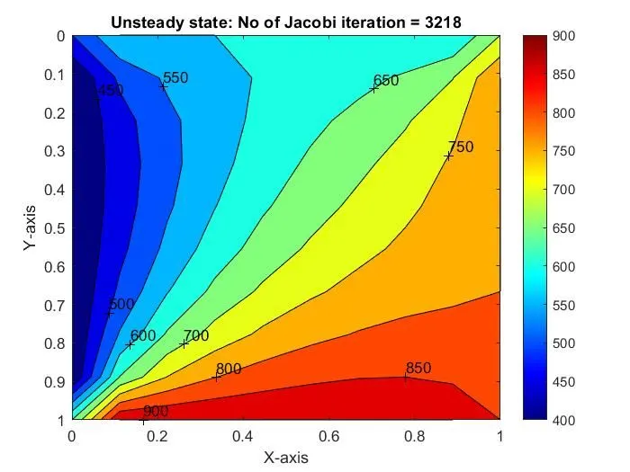
- Unsteady state - Jacobi iteration: (for input 1)
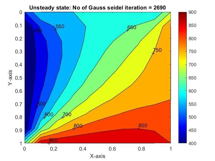
- Unsteady state - Gauss seidel: (for input 2)
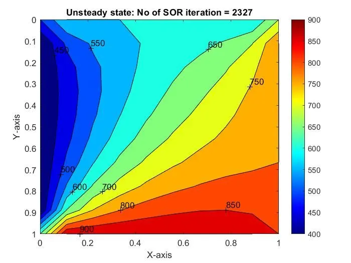
- Unsteady state - SOR method: (for input 3)
- Unsteady state - Explicit method:
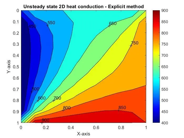
Conclusion:
- From the above simulation it is observed that in Implicit method, no of iterations that took to converge to the result is more for Jacobi followed by Gauss seidel and SOR respectively
- that is SOR is speeding up the process of converge of JAcobi and gauss seidel
- Hence it is optimal to use SOR metod for complex problems
- the relaxation parameter needs to be chosen optimally and it has some methods to find the optimum relaxation parameter, else the result will be dangling around the answer hence it will take more iterations.
- Hence from this analysis, we can observe that on the basis of simulation time, Jacobi iteration>Gauss seidel>SOR