Week 3.5 - Deriving 4th order approximation of a 2nd order derivative using Taylor Table method

Aim:

To compute the 4th order approximations of the second order derivative by central and skewed schemes and compare the errors from the respective schemes and understand the importance of different schemes

Explanation:

For any order of approximation of any order derivative can be computed using taylor table method. different types of schemes are employed to find the numerical value of the function.
Taylor table is used to find the coefficients of the hypothesis function
Taylor expansion for `f(x+dx) =f(x)+f'(x)Deltax+(f''(x))/(2!)Deltax^2+ (f'''(x))/(3!)Deltax^3+(f^(iv)(x))/(4!)Deltax^4.....`

1. Central difference scheme:

For central schemes, the number of nodes to be considered is given by the expression, nodes (`n`)= order of approximation (`p`) + order of derivative (`q`) - 1

In our case, `p` = 4 and `q` = 2, hence `n` = 4+2-1 = 5 , ie 5 nodes equispaced by distance dx. The 5 nodes are (i-2), (i-1), (i), (i+1), (i+2)

`:.` the hypothesis equation is given by, `Deltax^2 (d^2f)/(dx^2) ~~ af(i-2)+bf(i-1)+cf(i)+df(i+1)+ef(i+2)`
Taylor's table for above eqn is given by

	`f(x)`	`Deltax f'(x)`	`Deltax^2 f''(x)`	`Deltax^3 f'''(x)`	`Deltax^4 f^(iv)(x)`	`Deltax^5 f^(v)(x)`	`Deltax^6 f^(vi)(x)`
`af(i-2)`	`a`	`-2a`	`2a`	`-a4/3`	`a2/3`	`-a4/15`	`a4/45`
`bf(i-1)`	`b`	`-b`	`b/2`	`-b/6`	`b/24`	`-b/120`	`b/720`
`cf(i)`	`c`	`0`	`0`	`0`	`0`	`0`	`0`
`df(i+1)`	`d`	`d`	`d/2`	`d/6`	`d/24`	`d/120`	`d/720`
`ef(i+2)`	`e`	`2e`	`2e`	`e4/3`	`e2/3`	`e4/15`	`e4/45`
Sum of coefficients	`0`	`0`	`1`	`0`	`0`	Not known	Not known

From the taylor table, we have 5 algebraic equations with 5 unknowns,

`a+b+c+d+e=0`-------------- (1)
`-2a-b+d+2e=0`-------------- (2)
`2a+b/2+d/2+2e=1`------------ (3)
`-a4/3-b/6+d/6+e4/3=0`------- (4)
`a2/3+b/24+d/24+e2/3=0`----- (5)

Convert into matrix form,

A =`[[1,1,1,1,1],[-2,-1,0,1,2],[2,1/2,0,1/2,2],[-4/3,-1/6,0,1/6,4/3],[2/3,1/24,0,1/24,2/3]]`X =`[[a],[b],[c],[d],[e]]` B =`[[0],[0],[1],[0],[0]]`

X=A\B or A^-1*B (In matlab operation)

Solving the equation,

`a`= -0.0833
`b`= 1.3333
`c`= -2.5000
`d`= 1.3333
`e`= -0.0833

Substituting in the colum 7 and 8 we know that, 7th column will equals to 0 and 8 column will not be equals to zero
Rewriting the hypothesis equation, we get that
`Deltax^2 (d^2f)/(dx^2) ~~ af(i-2)+bf(i-1)+cf(i)+df(i+1)+ef(i+2)`= `Deltax^2f''(x)+Deltax^6(2*(4/45*a+b/720))`

Divide by `Deltax^2`on both sides, then the order of the leading term of the truncation error is `Deltax^4`
Hence it called as fourth order approximation of the first order derivative.
`:.` The formula of the numerical expression is given by `(-1f(i-2)+16f(i-1)-30f(i)+16f(i+1)-1f(i+2))/(12Deltax^2)`

2. Skewed right side scheme:

For skewed schemes, the number of nodes to be considered is given by the expression, nodes (`n`)= order of approximation (`p`) + order of derivative (`q`)
In our case, p=4 and q=2 hence n=4+2=6, the six nodes are given as (i), (i+1), (i+2), (i+3), (i+4), (i+5)

`:.` The hypothesis equation is given as, `Deltax^2 (d^2f)/(dx^2) ~~ af(i)+bf(i+1)+cf(i+2)+df(i+3)+ef(i+4)+gf(i+5)`

	`f(x)`	`Deltax f'(x)`	`Deltax^2 f''(x)`	`Deltax^3 f'''(x)`	`Deltax^4 f^(iv)(x)`	`Deltax^5 f^(v)(x)`	`Deltax^6 f^(vi)(x)`
`af(i)`	`a`	`0`	`0`	`0`	`0`	`0`	`0`
`bf(i+1)`	`b`	`b`	`b/2`	`b/6`	`b/24`	`b/120`	`b/720`
`cf(i+2)`	`c`	`2c`	`2c`	`c4/3`	`c2/3`	`c4/15`	`c4/45`
`df(i+3)`	`d`	`3d`	`d9/2`	`d27/6`	`d81/24`	`d243/120`	`d729/720`
`ef(i+4)`	`e`	`4e`	`e16/2`	`e64/6`	`e256/24`	`e1024/120`	`e4096/720`
`gf(i+5)`	`g`	`g5`	`g25/2`	`g125/6`	`g625/24`	`g3125/120`	`g15625/720`
Sum of coefficients	`0`	`0`	`1`	`0`	`0`	`0`	Not known

From taylor table, we can obtain 5 quadratic equations,

`a+b+c+d+e+g=0`-------------- (1)
`b+2c+3d+4e+5g=0`-------------- (2)
`b/2+2c+9/2d+16/2e+25/2g=1`-------------- (3)
`b/6+c4/3+d27/6+e64/6+g125/6=0`-------------- (4)
`b/24+c2/3+d81/24+e256/24+g625/24=0`-------------- (5)
`b/120+c4/15+d243/120+e1024/120+g3125/120=0`-------------- (6)

Converting into matrix form,

A=`[[1,1,1,1,1,1],[0,1,2,3,4,5],[0,1/2,2,9/2,16/2,25/2],[0,1/6,4/3,27/6,64/6,125/6],[0,1/24,2/3,81/24,256/24,625/24],[0,1/120,4/15,243/120,1024/120,3125/120]]`X =`[[a],[b],[c],[d],[e],[g]]` B =`[[0],[0],[1],[0],[0],[0]]`

Solving the equation, we get

`a`=`3.7500`
`b`=`-12.8333`
`c`=`17.8333`
`d`=`-13.0000`
`e`=`5.0833`
`g`=`-0.8333`

Substituting the values in hypothesis equation, we get
`Deltax^2 (d^2f)/(dx^2) ~~ af(i)+bf(i+1)+cf(i+2)+df(i+3)+ef(i+4)+g(i+5)`= `Deltax^2f''(x)+f^(vi)*Deltax^6`

Divide by `Deltax^2`on both sides, then the order of the leading term of the truncation error is `Deltax^4`
Hence it called as fourth order approximation of the first order derivative.
`:.` The formula of the numerical expression is given by `(3.75f(i)-12.8333f(i+1)+17.8333f(i+2)-13f(i+3)+5.0833f(i+4)-0.8333f(i+5))/(Deltax^2)`

3.Skewed left side scheme:

For skewed schemes, the number of nodes to be considered is given by the expression, nodes (`n`)= order of approximation (`p`) + order of derivative (`q`)
In our case, p=4 and q=2 hence n=4+2=6, the six nodes are given as (i-5), (i-4), (i-3), (i-2), (i-1), (i)

`:.` The hypothesis equation is given as, `Deltax^2 (d^2f)/(dx^2) ~~ af(i-5)+bf(i-4)+cf(i-3)+df(i-2)+ef(i-1)+gf(i)`

	`f(x)`	`Deltax f'(x)`	`Deltax^2 f''(x)`	`Deltax^3 f'''(x)`	`Deltax^4 f^(iv)(x)`	`Deltax^5 f^(v)(x)`	`Deltax^6 f^(vi)(x)`
`af(i-5)`	`a`	`-a5`	`a25/2`	`-a125/6`	`a625/24`	`-a3125/120`	`a15625/720`
`bf(i-4)`	`b`	`-4b`	`b16/2`	`-b64/6`	`b256/24`	`-b1024/120`	`b4096/720`
`cf(i-3)`	`c`	`-3c`	`9/2c`	`-c27/6`	`c81/24`	`-c243/120`	`c729/45`
`df(i-2)`	`d`	`-2d`	`d2`	`-d8/6`	`d16/24`	`-d32/120`	`d64/720`
`ef(i-1)`	`e`	`-e`	`e/2`	`-e/6`	`e/24`	`-e/120`	`e/720`
`gf(i)`	`g`	`0`	`0`	`0`	`0`	`0`	`0`
Sum of coefficients	`0`	`0`	`1`	`0`	`0`	`0`	Not known

From taylor table, we can obtain 5 quadratic equations,

`a+b+c+d+e+g=0`-------------- (1)
`-(5a+4b+3c+2d+e+0)=0`-------------- (2)
`25a/2+16b/2+c9/2+d2+e/2+0=1`-------------- (3)
`-(a125/6+b64/6+c27/6+d8/6+e/6+0)=0`-------------- (4)
`a625/24+b256/24+c81/24+d16/24+e/24+0=0`-------------- (5)
`-(a3125/120+b1024/120+c243/120+d32/120+e/120+0)=0`-------------- (6)

Converting into matrix form,

A=`[[1,1,1,1,1,1],[-5,-4,-3,-2,-1,0],[25/2,16/2,9/2,2,1/2,0],[-125/6,-64/6,-27/6,-8/6,-1/6,0],[625/24,256/24,81/24,16/24,1/24,0],[-3125/120,-1024/120,-243/120,-32/120,-1/120,0]]`X =`[[a],[b],[c],[d],[e],[g]]` B =`[[0],[0],[1],[0],[0],[0]]`

Solving the equation, we get

`a`=`-0.8333`
`b`=`5.0833`
`c`=`-13.0000`
`d`=`17.8333`
`e`=`-12.8333`
`g`=`3.7500`

Substituting the values in hypothesis equation, we get
`Deltax^2 (d^2f)/(dx^2) ~~ af(i-5)+bf(i-4)+cf(i-3)+df(i-2)+ef(i-1)+g(i)`= `Deltax^2f''(x)+f^(vi)*Deltax^6`

Divide by `Deltax^2`on both sides, then the order of the leading term of the truncation error is `Deltax^4`
Hence it called as fourth order approximation of the first order derivative.
`:.` The formula of the numerical expression is given by, `(3.75f(i)-12.8333f(i-1)+17.8333f(i-2)-13f(i-3)+5.0833f(i-4)-0.8333f(i-5))/(Deltax^2)`

Matlab program:

______________________________________________________________________________________clear all
close all
clc

%function we are computing is f(x) = sin(x)/x^3 for x=pi/3 and dx=pi/30
%Compare the errors for different schemes

%analytical derivative of second order
x=pi/3;
a=20;
dx=linspace(pi/4,pi/4000,a);
analytical_derivative = -2*exp(x)*sin(x);

%pre defining the size of the variables inorder to allocate memory while
%compiling
central_differencing = zeros(a,1);
skewed_right = zeros(a,1);
skewed_left = zeros(a,1);
error_central_diff = zeros(a,1);
error_skewed_right = zeros(a,1);
error_skewed_left = zeros(a,1);

for i=1:length(dx)
%function will be called to compute the fourth order approximations of
%the second order derivative for different differencing schemes
 [central_differencing(i),skewed_right(i),skewed_left(i)]  = scheme_dx(x,dx(i));

 %Truncation error central differencing scheme
error_central_diff(i)= abs(analytical_derivative-central_differencing(i));

%Truncation error right skewed differencing scheme
error_skewed_right(i)= abs(analytical_derivative-skewed_right(i));

%Truncation error left skewed differencing scheme
error_skewed_left(i)= abs(analytical_derivative-skewed_left(i));

end

%Log plot of dx vs truncation error
figure(1)
loglog(dx,error_central_diff,'LineWidth',1.5)
hold on
loglog(dx,error_skewed_right,'r','LineWidth',1.5)
hold on 
loglog(dx,error_skewed_left,'g','LineWidth',1.5)
xlabel('Range of dx')
ylabel('Truncation error')
title('Truncation error analysis on lograthamic scale')
legend('Central differencing error','Skewed right differencing error','Skewed left differencing error')
______________________________________________________________________________________

This above program will compute analytical and numerical value for the second derivative of fourth order approximation of the function f(x) = exp(x)*cos(x)
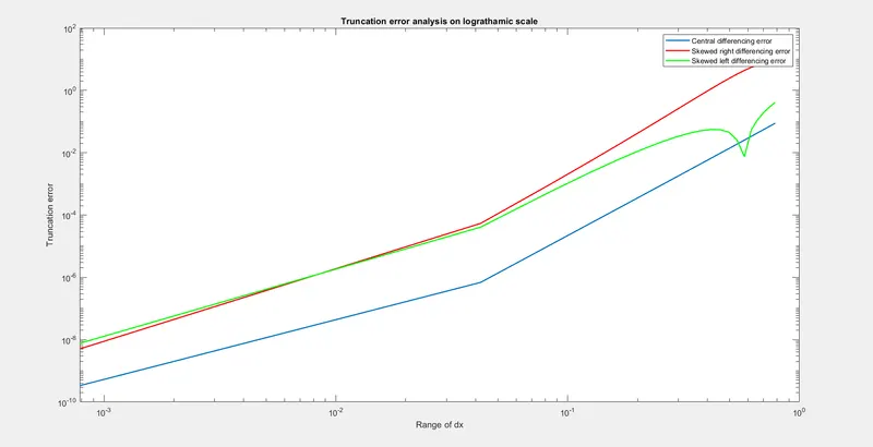
The error for each scheme is compared using log log plot.

Function:

______________________________________________________________________________________
function [a,b,c] = scheme_dx(x,dx)

%Fourth order approximation of the second order derivative
%function to be computed is f(x)= exp(x)*cos(x)

%central differencing scheme
% It is given by the expression f''(x) = (-f(i-2)+16f(i-1)-6f(i)+16f(i+1)-f(i+2))/(12dx^2)
a = ((-exp(x-2*dx)*cos(x-2*dx))+(16*(exp(x-dx)*cos(x-dx)))-(30*(exp(x)*cos(x)))+(16*(exp(x+dx)*cos(x+dx)))+(-exp(x+2*dx)*cos(x+2*dx)))/(12*dx^2);

%Skewed right differencing scheme 
% It is given by the expression f''(x) = (3.75f(i)-12.8333f(i+1)+17.8333f(i+2)-13f(i+3)+5.0833f(i+4)-0.8333f(i+5))/(dx^2)
% b = (3.75*(exp(x)*cos(x))-12.8333*(exp(x+dx)*cos(x+dx))+17.8333*(exp(x+2*dx)*cos(x+2*dx))-13*(exp(x+3*dx)*cos(x+3*dx))+5.0833*(exp(x+4*dx)*cos(x+4*dx))-0.8333*(exp(x+5*dx)*cos(x+5*dx)))/dx^2;
b = (45*(exp(x)*cos(x))-154*(exp(x+dx)*cos(x+dx))+214*(exp(x+2*dx)*cos(x+2*dx))-156*(exp(x+3*dx)*cos(x+3*dx))+61*(exp(x+4*dx)*cos(x+4*dx))-10*(exp(x+5*dx)*cos(x+5*dx)))/(12*dx^2);

%Skewed left differencing scheme
% It is given by the expression f''(x) = (3.75f(i)-12.8333f(i-1)+17.8333f(i-2)-13f(i-3)+5.0833f(i-4)-0.8333f(i-5))/(dx^2)
% c = (3.75*(exp(x)*cos(x))-12.8333*(exp(x-dx)*cos(x-dx))+17.8333*(exp(x-2*dx)*cos(x-2*dx))-13*(exp(x-3*dx)*cos(x-3*dx))+5.0833*(exp(x-4*dx)*cos(x-4*dx))-0.8333*(exp(x-5*dx)*cos(x-5*dx)))/dx^2;
c = (45*(exp(x)*cos(x))-154*(exp(x-dx)*cos(x-dx))+214*(exp(x-2*dx)*cos(x-2*dx))-156*(exp(x-3*dx)*cos(x-3*dx))+61*(exp(x-4*dx)*cos(x-4*dx))-10*(exp(x-5*dx)*cos(x-5*dx)))/(12*dx^2);

end
______________________________________________________________________________________

The coefficients in the numerical formula is given as fractions instead of decimals, coz even the ignored decimal values will generate an error in the value
Hence it is a good practice of using the fractions instead of decimal points.
When the program is computed, then we may obtain the plot from which we can understand the error of different schemes

Conclusion:

From the plot we can undertand that, central differencing error is much lower than the other cases, i.e. central differencing scheme provides the most accurate ans in this case.
In some other cases, skewed differencing scheme is more useful that central differencing scheme.
Central differencing scheme requires information from front and back where as if are solving the equation at boundary, then it is not possible to get info from front and back, hence skewed differencing are useful at that conditions.