Week 4 - CHT Analysis on Exhaust port

OBJECTIVES

The aim is to conduct a CHT Analysis on an Exhaust port model. The problem statements to put into consideration are:

1. Give a brief description of why and where a CHT analysis is used.
2. Maintain the y+ value according to the turbulence model and justify the results.
3. Calculate the wall/surface heat transfer coefficient on the internal solid surface & show the velocity & temperature contours in appropriate areas.
4. How would you verify if the HTC predictions from the simulations are right? On what factors does the accuracy of the prediction depend on?

What is CHT analysis? Why and where is it used?

Conjugate Heat Transfer (CHT) is the coupled heat transfer wherein the heat conduction in solids and the convective and radiative effects in surrounding fluids are taken into account. This is because, in solids, conduction mode dominates whereas in fluids convection and radiation modes dominate. Effectively combining both the effects in solid- fluid heat transfer systems is the key to its designing.

Heat transfers in solid and fluid are combined in many applications. CHT analysis is used in cases where variations in temperatures in solid and fluid parts occur due to the thermal interaction between the solid-fluid interfaces. The physics of conjugate heat transfer is common in different engineering applications such as HVAC, heat exchangers, electronic component design.

CHT Analysis on an Exhaust port model

• Geometry

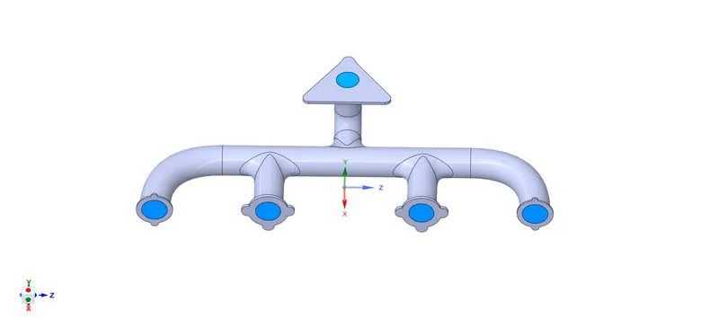
The figure shows the model of a 4 cylinder engine exhaust manifold. The fluid volume extracted is shown in blue. The fluid and solid volumes are shared using share topology inorder to obtain a conformal mesh. There are 4 inlets and 1 outlet port.

• Mesh generated

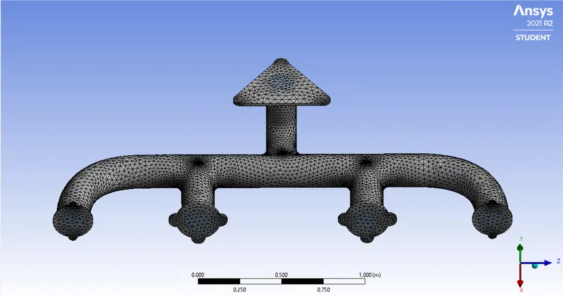
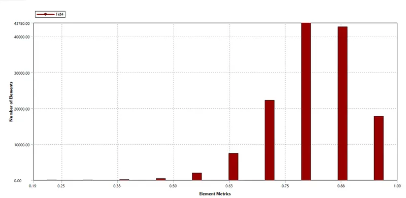
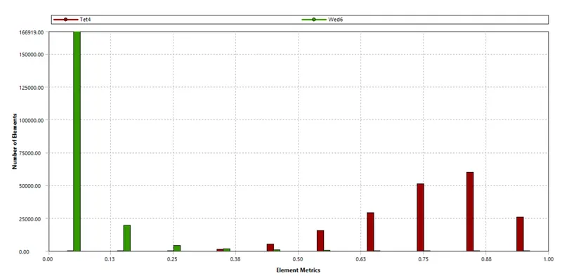
Case 1: The geometry is opened in the meshing console and a baseline mesh is generated initially. 136078 elements are produced in this case. The element quality metrics is given below.

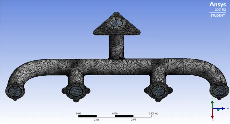
Case 2: The mesh is refined further to produce effective simulation results. The mesh is finer at the solid part, having 379835 elements. 8 inflation layers with a growth rate of 1.2 and total thickness of 5 e-003m was given.

• Pre-processing setup

The material used as solid is aluminium and as fluid is air. The turbulence model selected is standard k-epsilon model.

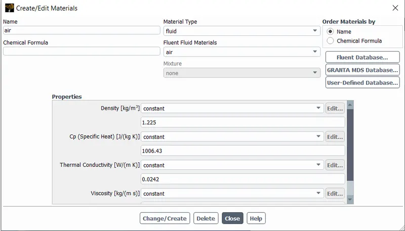
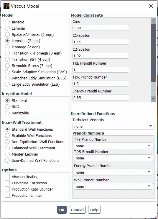
The boundary conditions are given to the mesh. Inlet velocity is given to be 50m/s and the temperatre as 700K.

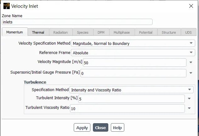
The outlet is given a pressure outlet boundary condition. The pressure is set to a 0 gauge pressure value. The outer wall of the solid is assigned a convection thermal condition with a heat transfer coefficient of 20W/(m^2 K). All the other walls are kept as isothermal.

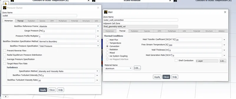
The setup is then initialised according to the hybrid initialising method and then solved for 500 iterations.

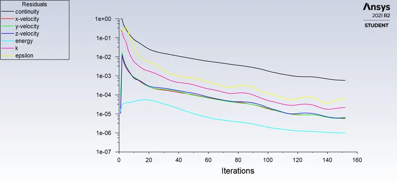
• Solution (Case 1 Baseline mesh: Residual plot and temperature contour of the system)

Solution converged at 152th iteration.

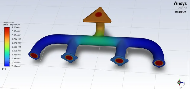
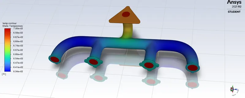
• Solution (Case 2 Refined mesh: Residual plot and temperature contour of the system)

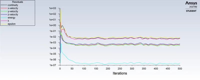
• Results

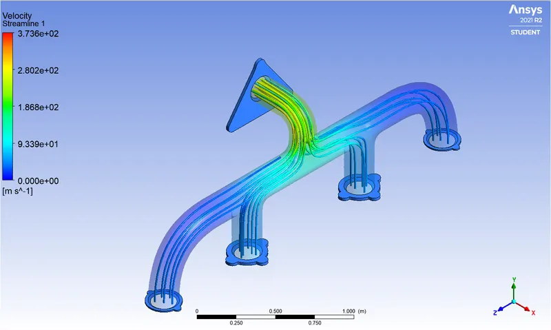
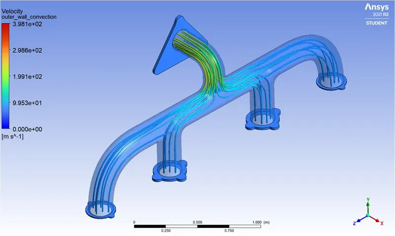
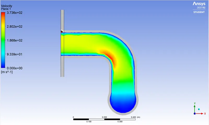
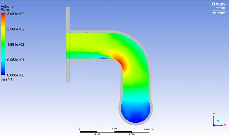
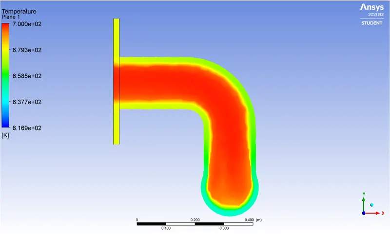
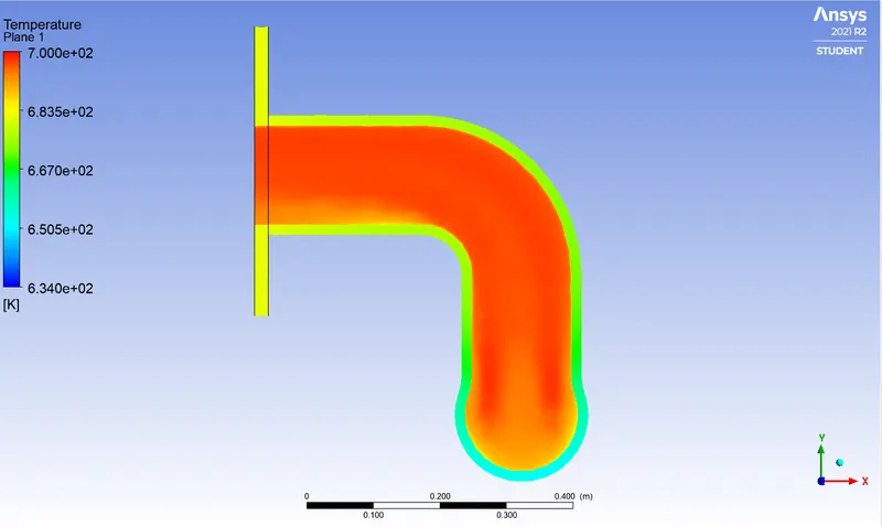
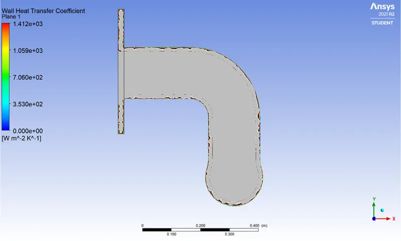
Inorder to find the changes that occur while refinement of the mesh, following comparisons are made on the velocity contour, temperature contour and wall heat transfer coefficient. The figure in the left shows the respective result of the baseline mesh whereas the right shows the results from the refined mesh.

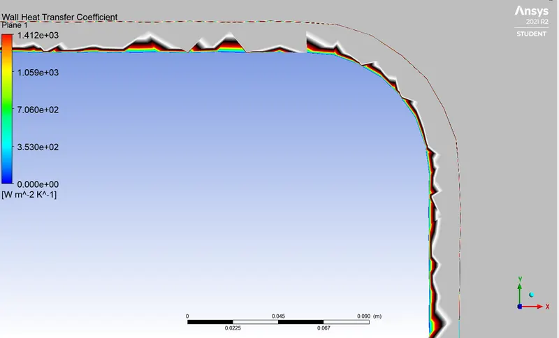
On refining the mesh, it is observed that the plot becomes more smooth neat the inner boundary and hence the results become more accurate with a notable increase in their values.

Baseline mesh Refined mesh

Velocity streamlines

Velocity contour

Temperature contour

Wall Heat Transfer Coefficient contour

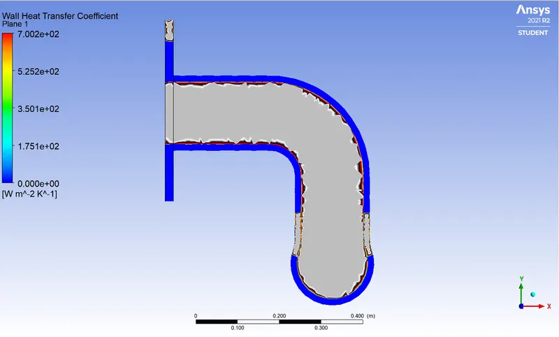
Enlarged view of the wall heat transfer coefficient contour in refined mesh.

How would you verify if the HTC predictions from the simulations are right? On what factors does the accuracy of the prediction depend on?

We can find the heat transfer coefficient (HTC) from Nusselt number equation. Hence,

`h=(Nu.k)/L` where,

`Nu=`Nusselt number, `k=`Thermal conductivity, `L=`Characteristic length

Nusselt number is the function of Reynolds Number which is inturn directly proportional to velocity ie., Nusselt number is directly proportional to velocity and so is the heat transfer coefficient.

`Nu=0.664*Re^0.5*Pr^0.33` and `Re=(rho*v*L)/mu`

Factors on which prediction accuracy depends on:

• The finer the mesh, the more accurate the results.
• The presence of inflation layers at the boundary improves the quality and thus capture the variations effectively.
• The mesh at the solid fluid interface must be strictly conformal.

CONCLUSIONS

1. CHT analysis was successfully conducted on baseline and refined meshes.
2. The maximum velocity for baseline case is 373.6m/s and for refined mesh 398.1is m/s.
3. The wall heat transfer coefficient was found to be 1412 W/(m^2 K).